Use Multiple Worksheets to Create 3D Excel Charts

A 3D Excel formula allows you to calculate cells across multiple worksheets. It is incredibly useful for creating a summary sheet to share data with others. You can then share the results visually with the help of a 3D Excel Chart.

Download and follow along with 3D Excel Charts.xlsx.

Step-by-Step: 3D Excel Formula

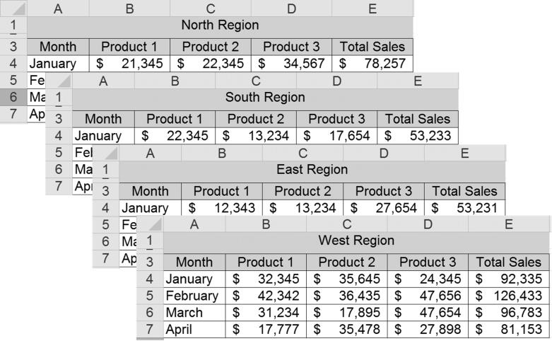
1. Make sure that all of your worksheets are set-up exactly the same. You want them to have the same type of data in the same / corresponding cells.
2. Create a summary page.
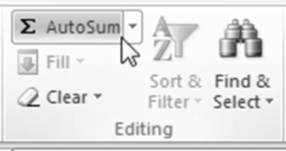
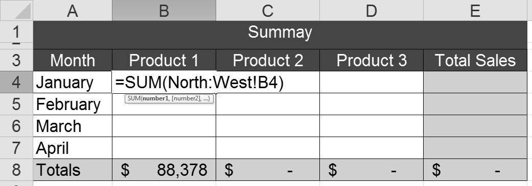
3. Select the first cell and click the AutoSum button on the Home tab (or create any other type of formula).
4. Select the first worksheet tab you wish to include.
5. Click the corresponding cell in that sheet.
6. Hold down Shift.
7. Select the last worksheet tab you wish to include.
8. Hit Enter.
9. Use the AutoFill Handle to copy the formula to the rest of the Summary spreadsheet.

Give it a Try!

Rather than go through this manual process, you can use the worksheet names to design your formula in the formula bar.

 Add a 3D Excel Chart

You can now select your data and translate your summary into a dynamic chart.

Step-by-Step: 3D Excel Chart

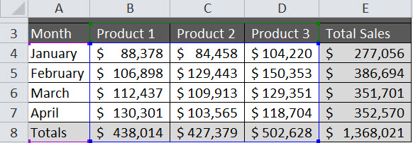
1. Select your chart data range. In this example, we used $A$3:$D$8 to show Month, Product type, and Totals data.
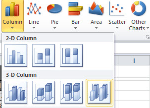
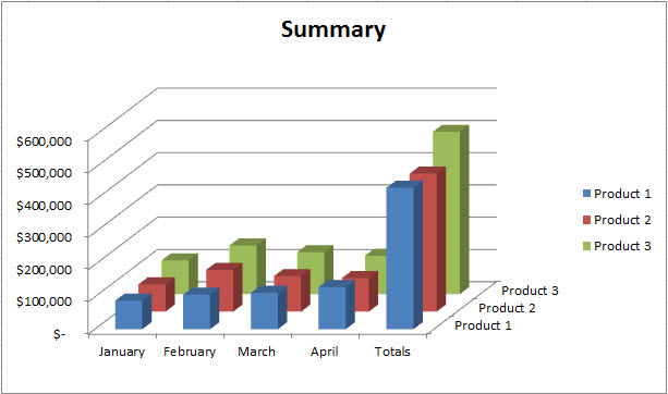
2. On the Insert tab, choose the Column dropdown in the Charts You can now choose a 3D chart type for your Summary data. This example shows the 3D Column chart type, but there are many 3D Excel charts to choose from. Choose the best for your data and audience!