How to Create a Dynamic Named Range in Excel for Rolling Charts

Key Takeaways

• A dynamic named range in Excel automatically adjusts to include new data, eliminating the need to manually update chart references.

• The OFFSET function combined with COUNT lets you build a rolling chart that always displays a specific number of recent data points such as the last 12 months.

• Once you assign a dynamic named range to a chart's data source, the chart refreshes itself whenever you add new rows to your dataset.

• You can edit dynamic named ranges at any time through Name Manager on the Formulas tab.

What Is a Dynamic Named Range in Excel?

A dynamic named range in Excel is a named reference that automatically adjusts its boundaries as your data grows or shifts. Unlike a static named range, which points to a fixed set of cells (such as B1:B12), a dynamic named range uses a formula to expand or contract based on the actual data in your worksheet. You can create a dynamic named range using the OFFSET function, the INDEX function or a combination of other formulas.

This technique is especially useful for charts, data validation drop-downs and formulas that reference growing datasets. Instead of manually editing cell references every time you add a row, the named range handles the update for you.

Why Use a Dynamic Named Range for Rolling Charts

Creating reports on a regular schedule is a common task for the business Excel user. When you need to create a Rolling chart that reflects data in a specific timeframe – such as the previous 12 months - you can quickly find yourself in a maintenance nightmare, updating your charts manually to include the new month's data and exclude the now "out of date" data. The good news is that with the OFFSET function, you can create a dynamic rolling chart that automatically refreshes your charts far more easily than adjusting cell references or deleting the old data.

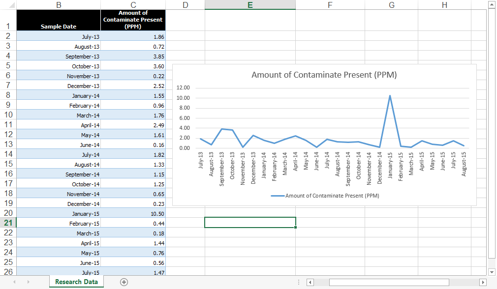
The following steps demonstrate how to use the OFFSET function to create an annual rolling chart. We have a table that shows amounts of contaminate present in an imaginary water sample taken monthly. We want a chart that shows the current month's data along with the previous 11 months. To follow using our example below, download Excel Rolling Chart.xlsx

Our initial chart shows two years of data.

Before You Begin

Before diving into the steps, make sure you have the following in place:

• Excel version: Excel 2010 or later or Microsoft 365

• Sample file: If you haven't already, download the sample file linked above to follow along with the tutorial

• Data layout: Your data should be organized in a contiguous table with headers in the first row

• Cursor position: Place your cursor in an empty cell before defining names so Excel does not auto-select existing data

Specify a Dynamic Named Range

First, create a dynamic named range for the data that uses the OFFSET function to make it reflect a relative timeframe:

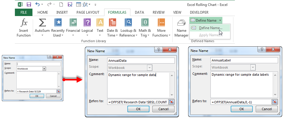
1. Make sure your cursor is in an empty cell and no data in your table is selected to begin, then select Define Name on the Formulas tab to open the New Name dialog box.

2. Give the range a recognizable name in the Name field. A name must use the following syntax:

   • First character can only be a letter, an underscore "_" or a backslash "\"

   • You can use letters, numbers, periods, and underscores in the rest of the name, but NOT spaces. Names are NOT case sensitive – "DATA" will be seen as the same as "data"

   • Names cannot be the same as a cell reference

In this example our named range is AnnualData. (Note: if you want to follow along and create a new chart of your own, type your own range name in the textbox and substitute that name in the formulas below. See also Changing Names in the bonus paragraph at the end of this article.)

3. In the Refers to: text field, replace the default cell reference with your OFFSET function. The syntax for OFFSET is:

OFFSET(reference, rows, cols, [height], [width])

so the formula for our dynamic named range's data will be

=OFFSET('Research Data'!$B$1,COUNT('Research Data'!$B:$B),0,-12,1)

Notice that the COUNT function gives us a total number of rows in our table, and we then specify how many rows we want to include in the [height] argument. This is where you can change the number of months (for example) you want to include in your chart. If, instead, you added columns to your data each month, you would adjust your formula accordingly.

HINT! Excel will try to be "helpful" and add cell references or ranges to the Refers to: text field if you click on something outside of the dialog box. You may have to type or paste very carefully into this text box to avoid "extra" data in your formulas.

4. Create a named range for the labels following the same steps above. The formula for our labels will be: =OFFSET(AnnualData,0,-1) We can use the range we created for the data as our reference and subtract 1 from our width to capture the correct range.

ssign Chart Data Source to Dynamic Named Range

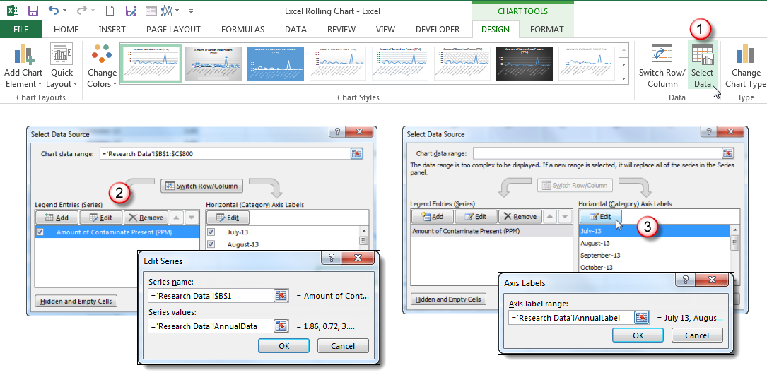
Create your line chart as you normally would if you have not already. Now, you need to tell the chart to use our dynamic range instead of the entire table. Click on the chart to activate the Chart Tools contextual tabs.

1. On the Design tab, click Select Data.

2. In the Select Data Source dialog box, select the first data series and click Edit.

   • In the Series values text box in the Edit Series dialog box, replace the default table range with the dynamic data named range. Do not change the sheet name and exclamation (!) that precedes it.

   • Click OK

3. Click on any label in the Horizontal (Category) Axis Labels selection box, then click Edit.

   • In the Axis Labels dialog box, replace the default range with the dynamic label named range.

   • Click OK.

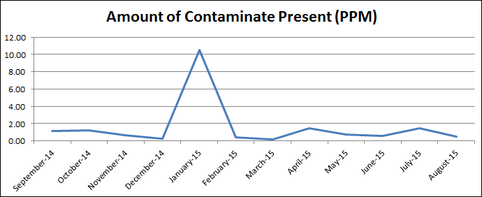
Now your chart will only show the last 12 rows of data.

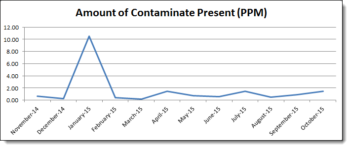
When you update your data by adding more rows, the chart will automatically show the new last 12 rows of data, creating a rolling chart effect.

Note that if you want to show more than one series of data on your chart, you will need to create a named range and repeat the above process for each series! This might take you a little more time to set your charts up, but will save you much more in the long run as you simply add to your data and the chart does the rest.

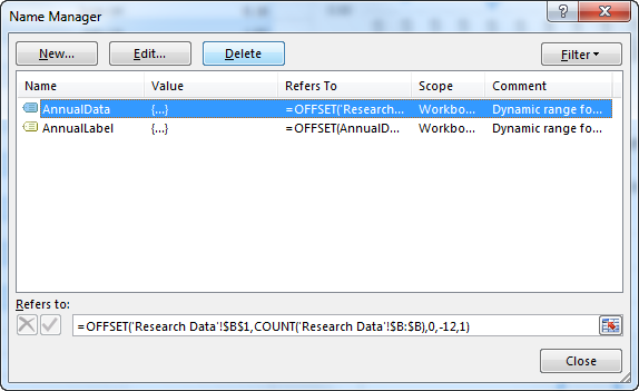ow to Edit a Dynamic Named Range

Once you have specified named items in your workbook, you may want to go back and edit them from time to time. Perhaps you want to change your OFFSET to show 6 months instead of 12, for example. To edit an existing name, click the Name Manager button on the Formulas tab. Select the name you wish to edit, then click the Edit button. Make your changes in the dialog box as you did when first creating it. Just be careful not to change the name itself if other formulas depend on it.

OPTIONAL: To check your work and compare named ranges, you can download Excel Rolling Chart_Complete.xlsx.

Alternative Methods for Creating Dynamic Named Ranges

The OFFSET function is the most common way to build a dynamic named range, but it is not the only option. Depending on your situation, one of these alternatives may work better.

1. Excel Table method: Format your data as an Excel Table by selecting your range and pressing Ctrl+T. When data is inside a Table, structured references automatically expand as you add new rows. This means charts and formulas tied to the Table update without any named range formula at all. For many use cases, this is the simplest approach.

2. INDEX with COUNTA: Instead of OFFSET, you can define a named range with a formula like =Sheet1!$B$1:INDEX(Sheet1!$B:$B,COUNTA(Sheet1!$B:$B)). This creates an expanding range that grows as you add data. The key advantage is that INDEX is a non-volatile function, meaning Excel only recalculates it when the referenced cells change. In large workbooks with many dynamic named ranges, switching from OFFSET to INDEX can noticeably improve performance.

Both methods produce a dynamic chart range that updates automatically. Choose the one that best fits your workbook size and reporting needs.

Troubleshooting Common Dynamic Named Range Issues

If your dynamic named range is not behaving as expected, check for these common problems:

• #REF! error: This typically appears when the named range formula references a sheet that has been deleted or renamed. Open Name Manager on the Formulas tab and verify that the sheet name in your formula matches the actual tab name in your workbook.

• Chart not updating: Make sure the dynamic named range was assigned directly as the chart's data source (not just defined in Name Manager). If the chart still points to a static cell range, it will not pick up the named range. Re-enter the named range in the Select Data Source dialog as described in the steps above.

• OFFSET returning wrong data: The COUNT function only counts cells containing numbers. If your column includes text or blank cells mixed in, COUNT may return an incorrect total. Use COUNTA instead if your data contains non-numeric values such as text labels.

• Excel auto-inserting cell references: When the New Name or Edit Name dialog box is open, clicking anywhere on the worksheet causes Excel to insert that cell reference into the Refers to field. Type or paste your formula carefully and avoid clicking outside the dialog until you are finished.

• Named range not visible in the Name Box: If you defined the named range with sheet-level scope instead of workbook scope, it will only appear when that specific sheet is active. To make it available across the entire workbook, recreate the name in Name Manager and set the Scope dropdown to Workbook.