Excel Conditional Formatting Formulas: How to Use If Statements

Key Takeaways

• Every conditional formatting rule is inherently an if/then statement: if the condition evaluates to TRUE, then Excel applies the formatting you specify.

• To create an if/then/else effect (e.g., format red if above a threshold, green if below), you need to set up two separate conditional formatting rules rather than one.

• You can use formulas with functions like AND, OR and MONTH inside conditional formatting rules to build powerful, dynamic formatting based on multiple conditions or other cells' values.

• Understanding relative vs. absolute cell references is essential for conditional formatting formulas to apply correctly across a range.

What Is Conditional Formatting with a Formula in Excel

Conditional formatting is an Excel feature that automatically changes the appearance of cells based on conditions you define. While Excel offers built-in preset rules for common scenarios like highlighting cells greater than a specific value or flagging the top 10%, you can also write custom formulas to control exactly when formatting is applied. This is where the real power of an excel conditional formatting formula lies.

When you use a formula, you can reference other cells, combine conditions with AND or OR and use functions like MONTH(), TODAY() and VLOOKUP() to create dynamic, intelligent formatting. Every conditional formatting rule is fundamentally a conditional formatting if statement: if the formula evaluates to TRUE, then Excel applies the format. If it evaluates to FALSE, the formatting is not applied.

One important distinction: you cannot use the IF() function itself to return different formats within a single rule. Instead, you create separate rules for each condition you want to format differently. This guide walks through practical excel conditional formatting examples that show you how to build these rules step by step. For more about using dates in conditional formatting, see this article on conditional formatting with date data.

How to Create a Conditional Formatting Rule Using a Formula

Before jumping into specific scenarios, here is the general process for creating a conditional formatting formula rule. You can use a formula to determine which cells to format by following these steps:

1. Select the range of cells you want to format.

2. Go to Home > Conditional Formatting > New Rule.

3. Select "Use a formula to determine which cells to format."

4. Enter your formula in the formula field. The formula must return TRUE or FALSE.

5. Click Format to choose your formatting options (fill color, font color, borders, etc.).

6. Click OK to apply the rule.

You can apply multiple rules to the same range, which is how you create the effect of if/then/else logic. Each rule acts as its own if/then condition, and Excel evaluates them in order.

Understanding Cell References in Conditional Formatting Formulas

The most common source of confusion when writing a conditional formatting formula is how cell references behave. When you enter a formula in a conditional formatting rule, Excel uses relative and absolute references the same way it does in worksheet formulas, but the behavior can be surprising if you are not expecting it.

When you apply conditional formatting based on another cell, the type of reference you use determines whether the formula adjusts for each cell in the range or stays locked to one specific cell.

The key rule to remember: the cell reference in your formula should be relative to the first cell in your selected range. If your range starts at A1 and you want to check column A for every row, use =$A1. Excel will adjust the row number automatically as it evaluates each cell in the range.

Now that you understand the mechanics, let's walk through practical scenarios that demonstrate how to create the effect of if/then conditional formatting using custom formulas. To follow along using our examples, download 04-If-Then Conditional Formatting.xlsx.

If you are a fan of Excel's conditional formatting feature, you probably find yourself looking for even more ways to highlight useful information in your data. A question that often comes up among these "conditional formatting addicts" is: "Can I use an if/then formula to format a cell?"

The answer is yes and no. Any conditional formatting argument must generate a TRUE result, meaning that at a literal level, your conditional formatting rule is an If/Then statement along the lines of "If this condition is TRUE, THEN format the cell this way".

What conditional formatting can't do in a single rule is an IF/THEN/ELSE condition such as "If # is greater than 10, format red; else, format green." Instead, this would require TWO rules, one for "greater than 10" and one for "less than 10".

Let's look at a few scenarios to get a sense of how we can create the effect of IF/THEN conditional formatting, even if we can't use it in the feature itself:

Scenario 1 (Birthdays tab): You want to highlight employees who have a birthday this month. Employees in your department should be highlighted in red, and employees in all other departments should be highlighted in blue.

Solution: Create two rules – one for your department, one for all others

Step 1 – Highlight birthdays in your department

The formula to identify birthdays in the current month will be (see this article for more about using dates in conditional formatting):

=MONTH(C2)=MONTH(TODAY())

To create a formula that generates a TRUE/FALSE statement that highlights birthdays only in one department, you would use the formula:

=AND(MONTH(C2)=MONTH(TODAY()),D2="Sales")

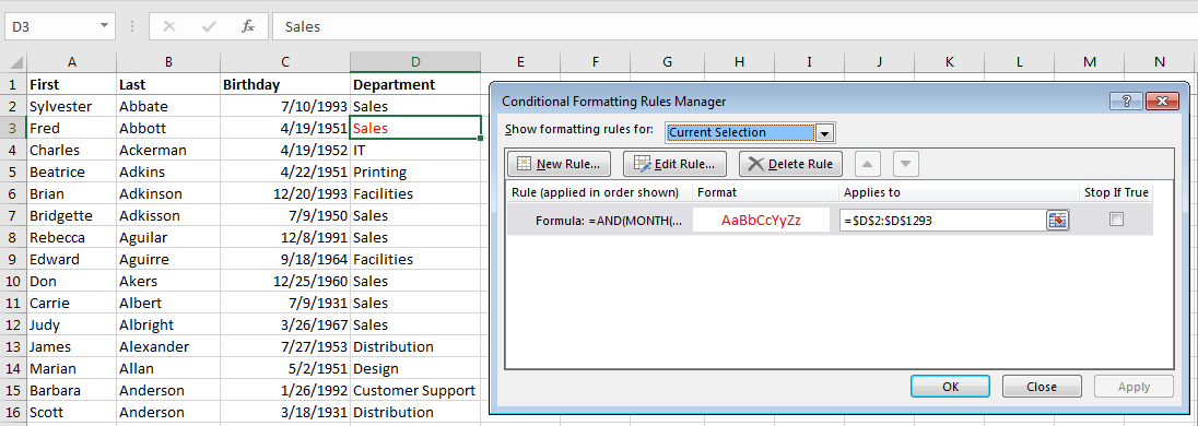
This example highlights birthdays in the current month, so your results will vary depending on when you follow along.

Then, create a second rule for the same range using this formula to highlight birthdays that are not in your department:

=AND(MONTH(C1)=MONTH(TODAY()),D1<>"Sales")

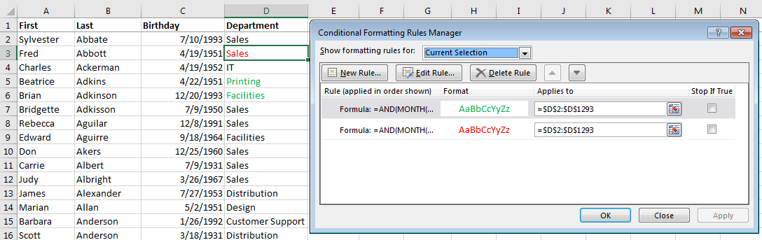
Bonus Tip

In this example, we applied the rule to the department cell to show the relationship to the formula. By changing the Applies to range, however, you can easily highlight a different cell – such as the birthdate – or the entire row. See Get the Most Out of Excel's Conditional Formatting for more ideas.

Scenario 2 (Retainers tab): You have a table of how many hours your employees have worked for specific clients, and you have a table of how many hours each client has in their retainer budget. You want to highlight the clients who are over their retainer.

Solution 1: Create a helper column using IF/THEN formula to call out whether a client is over their retainer budget. If your worksheet already has the IF/THEN/ELSE logic you need embedded in a cell, conditional formatting can act based on those results. You don't necessarily need to reproduce the logic in the rule itself.

In this example, we already have an IF/THEN formula that returns the result "YES" if our client is over their retainer budget. Our conditional formatting rule only has to look for the text string "YES" and apply the formatting when true.

Highlight the cell range, then click on Conditional Formatting > Highlight Cell Rules > Text that Contains to create the rule. Type YES in the Text that Contains dialog box.

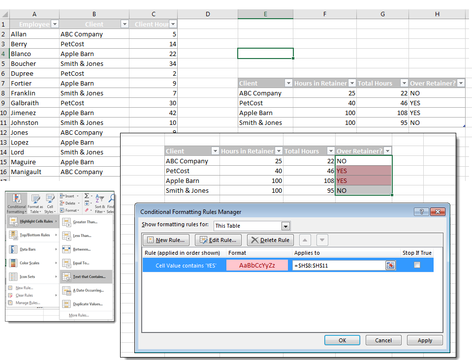
Solution 2: Create a formula to calculate retainer budget.

If you don't have, or don't want to create, a helper column with an IF/THEN statement, you can use the same method as the first scenario by creating a rule that determines whether a client is over budget. In this example, we applied the rule to the Client cells and the formula would be:

=(F8-G8)<0

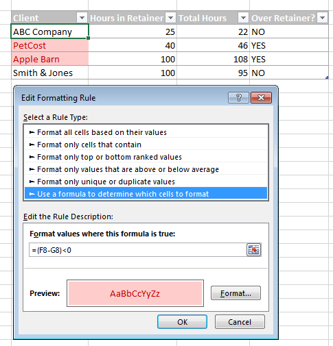
If you are used to creating complex formulas that cover all cases in one cell, it may take a little re-learning to figure out the approach for conditional formatting. The best hint is to remember that you can apply multiple rules to the same cells. Break up your formatting criteria into separate steps, and you'll most likely be able to get where you need to be! For more techniques like these, browse additional Excel tips and tutorials.

Troubleshooting Common Conditional Formatting Issues

Even with the right formula logic, conditional formatting rules can sometimes behave unexpectedly. Here are the most common issues and how to fix them:

• Formula returns unexpected results: Check whether you are using relative or absolute cell references. A relative reference like =A1>100 adjusts for each cell in the range, while =$A$1>100 locks to one cell. Review the cell references section above if you are unsure which to use.
• Formatting applies to wrong cells: Open the Rules Manager (Home > Conditional Formatting > Manage Rules) and verify the "Applies to" range. A mismatched range is one of the most frequent causes of unexpected formatting.
• Rule order matters: When multiple conditional formatting rules apply to the same range, Excel evaluates them from top to bottom. If a higher-priority rule is formatting cells first, your intended rule may never trigger. Use the "Stop If True" checkbox to prevent lower-priority rules from overriding.
• Formula errors (#REF!, #VALUE!): Ensure your formula references valid cells within the workbook. Also confirm that you are not using the IF() function expecting it to return a format. Conditional formatting formulas should return TRUE or FALSE, not text or numbers.
• Conditional formatting disappears after sorting or filtering: Rules tied to specific cell addresses may shift when data is rearranged. Use relative references so the rules adapt, or reapply your rules after sorting.

Tips for Managing Conditional Formatting Rules

As you build multiple conditional formatting rules across your worksheets, keeping them organized becomes important. Here are a few practical management tips:

• Edit an existing rule: Go to Home > Conditional Formatting > Manage Rules. Select the rule you want to modify, click Edit Rule and adjust the formula or formatting as needed.
• Reorder rules: In the Rules Manager, use the up and down arrows to change the priority order. Rules at the top of the list are evaluated first.
• Clear all rules: To remove conditional formatting from a selection or an entire sheet, go to Home > Conditional Formatting > Clear Rules and choose either "Clear Rules from Selected Cells" or "Clear Rules from Entire Sheet."
• Copy conditional formatting to other cells: Use the Format Painter tool on the Home tab. Select a cell with the formatting you want to copy, click Format Painter and then select the destination cells. This copies the conditional formatting rules along with other cell formatting.

Build Your Excel Skills with Pryor Learning

Pryor Learning offers live and on-demand Excel training covering conditional formatting, formulas, pivot tables, data analysis and more. With PryorPlus, you get unlimited access to the full library of Excel courses so you can keep building your skills at your own pace. Explore Pryor's Excel training options today.