How to Calculate Age in Excel: Formulas That Work

Key Takeaways

• The simplest way to calculate age in Excel is to subtract the birthdate from TODAY() and divide by 365.25, wrapped in INT() for a whole number.

• DATEDIF is the most flexible age formula in Excel, returning age in years, months, days or any combination.

• YEARFRAC provides a precise decimal age and works well for financial and compliance calculations.

• Always confirm date cells are formatted as dates (not text) to avoid calculation errors.

To calculate age in Excel, the quickest formula is =INT((TODAY()-B2)/365.25), where B2 contains the birthdate. This returns a whole number representing the person's current age in years.

Excel offers several methods to calculate age from a date of birth, and the right choice depends on how much precision you need. A simple subtraction formula works for quick estimates, while functions like YEARFRAC and DATEDIF provide more exact results, including breakdowns by years, months and days.

Whether you manage HR records, track employee eligibility or maintain compliance databases, this guide covers the basic subtraction method, YEARFRAC, DATEDIF, combined breakdowns, special use cases and troubleshooting to help you handle age calculations with confidence.

The Basic Age Formula in Excel

The fastest way to calculate age in Excel is with basic date arithmetic. This approach subtracts the birthdate from today's date and divides by 365.25 to account for leap years.

The formula looks like this: =INT((TODAY()-B2)/365.25), where B2 holds the birthdate.

Here is how to set it up:

1. Enter the birthdate in a cell (for example, B2). Make sure the cell is formatted as a date.

2. In an adjacent cell, type the formula =INT((TODAY()-B2)/365.25) and press Enter.

3. The cell displays the person's current age as a whole number in years.

The INT function rounds the result down to the nearest whole number, so you get complete years only. Keep in mind that this method is an approximation. Dividing by 365.25 accounts for most leap years, but it can occasionally be off by a day. For exact results, use DATEDIF or YEARFRAC as described in the sections below.

How to Calculate Age with YEARFRAC

YEARFRAC gives the number of years between two dates. The FRAC is short for fraction, because this function returns a number with a decimal representing the fractional portion of an incomplete year.

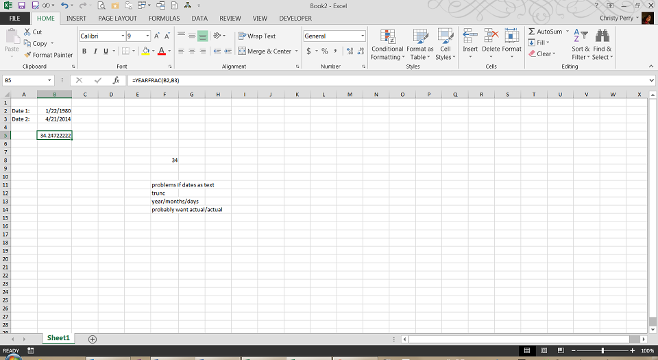
Many financial transactions assume that each month has 30 days and that each year has 360 days. Like other Excel finance formulas, YEARFRAC uses this "30/360" as the default method of calculating the number of years. In most cases this works well enough. However, if you prefer to use the actual number of days in each year, enter "1" for the optional third parameter.

To calculate a dynamic age that updates automatically, replace the second date with TODAY(). For example: =YEARFRAC(B2,TODAY()) returns the decimal age based on the current date.

YEARFRAC Syntax and Parameters

The full syntax is YEARFRAC(start_date, end_date, [basis]). Each parameter controls a part of the calculation:

• start_date: The beginning date (typically the birthdate).

• end_date: The ending date (such as TODAY() or a specific date).

• basis: An optional argument that defines the day-count method. The five options are:

  • 0 (or omitted): US (NASD) 30/360 - assumes 30-day months and 360-day years.

  • 1: Actual/actual - uses the real number of days in each month and year.

  • 2: Actual/360 - uses actual days but assumes a 360-day year.

  • 3: Actual/365 - uses actual days but assumes a 365-day year.

  • 4: European 30/360 - similar to option 0 with slight European convention differences.

For age calculations, basis 1 (actual/actual) gives the most precise result because it accounts for the true length of each year.

Getting Whole Years with INT or TRUNC

Note the .24722222 on the end of the number. This represents approximately a quarter of a year beyond the 34-year age. If you want only the number of complete years, wrap the formula in a TRUNC function: "=TRUNC(YEARFRAC(B2,B3))" returns an even 34.

You can also use INT to achieve the same result: =INT(YEARFRAC(B2,TODAY())). For positive numbers, INT and TRUNC behave identically - both remove the decimal portion and return the whole number of complete years. Either function works, but INT is more commonly used across Excel tutorials and documentation.

How to Calculate Age with DATEDIF

The DATEDIF function is a hidden function in Excel. It does not appear in the formula autocomplete list, but it is fully functional and widely used for age calculations.

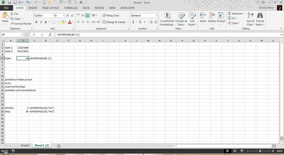
The "y" for the third parameter instructs Excel to count the number of years.

DATEDIF is more flexible than YEARFRAC. It calculates the number of years, months, or days, depending on the third parameter—"y" to calculate years, "ym" for months left over after the years are counted, and "md" for days left over after the years and months are counted.

The syntax is DATEDIF(start_date, end_date, unit). To calculate a person's current age, use =DATEDIF(B2,TODAY(),"Y"), where B2 contains the birthdate.

DATEDIF Unit Codes Explained

DATEDIF supports six unit codes, each returning a different piece of the date difference:

• "Y": The number of complete years between the two dates.

• "M": The total number of complete months between the two dates.

• "D": The total number of days between the two dates.

• "YM": The number of months remaining after complete years have been counted.

• "MD": The number of days remaining after complete years and months have been counted.

• "YD": The number of days remaining after complete years have been counted.

Important Notes about DATEDIF

There are a few things to keep in mind when using DATEDIF:

• The start_date must be earlier than or equal to the end_date. If the start date comes after the end date, DATEDIF returns a #NUM! error.

• Because DATEDIF is an undocumented function, it does not appear in Excel's formula autocomplete or function wizard. You must type the full formula manually.

• The "MD" unit code can occasionally return inaccurate results in certain Excel versions. If you need precise day counts, verify the output against a calendar or use an alternative calculation.

How to Calculate Age in Years, Months and Days

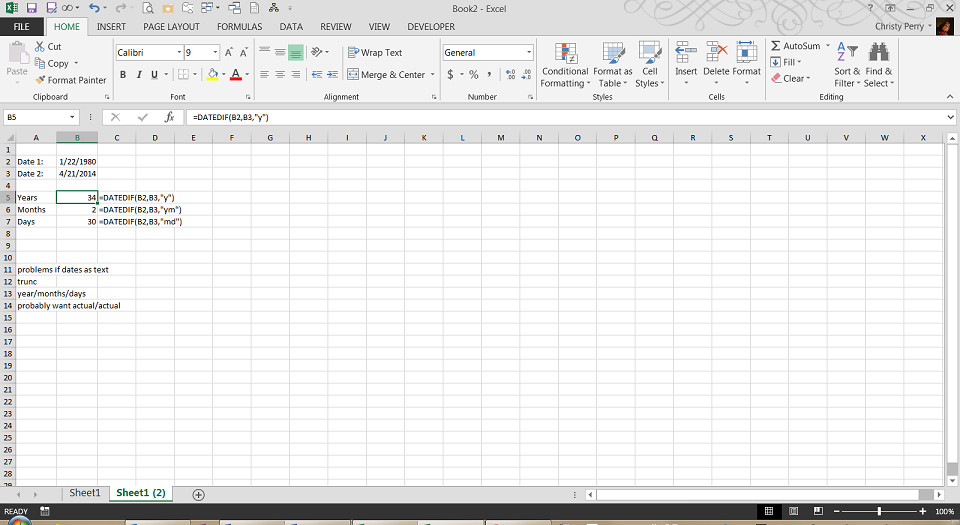
For a complete age breakdown, you can combine three DATEDIF calls into a single formula that displays years, months and days in a readable format. This is one of the most common ways to express age in years months and days in Excel, especially for HR and compliance records.

Follow these steps to build the combined formula:

1. Identify the cell containing the birthdate (for example, B2).

2. In an adjacent cell, enter the following formula: =DATEDIF(B2,TODAY(),"Y")&" years, "&DATEDIF(B2,TODAY(),"YM")&" months, "&DATEDIF(B2,TODAY(),"MD")&" days"

3. Press Enter. The cell displays a result like "34 years, 2 months, 30 days."

4. Note that this formula returns text, not a number, so you cannot use the result in further arithmetic without extracting the numeric portions separately.

This combined approach uses the "Y" code for complete years, "YM" for leftover months and "MD" for leftover days, concatenating them with the ampersand (&) operator.

Special Use Cases for Age Calculation

Beyond calculating a person's current age, Excel can handle several practical scenarios that come up regularly in HR, benefits administration and compliance work.

Calculating Age on a Specific Date

Sometimes you need to calculate age between two dates in Excel rather than using today's date. For example, you might need to know how old an employee was on their hire date or how old a participant will be on an event date.

Replace TODAY() with a cell reference or a typed date. For example: =DATEDIF(B2,D2,"Y"), where B2 is the birthdate and D2 is the target date. This returns the number of complete years between the two dates.

Calculating Age in a Certain Year

To determine how old someone will be (or was) at the start of a particular year, use the DATE function to build the target date. For example: =DATEDIF(B2,DATE(2025,1,1),"Y") returns the person's age as of January 1 of that year.

This is useful for benefits eligibility checks, retirement planning and annual compliance reporting where age must be evaluated at a fixed point in the calendar.

Finding the Date When Someone Reaches a Certain Age

You can also calculate the exact date when a person reaches a milestone age. The formula =DATE(YEAR(B2)+N,MONTH(B2),DAY(B2)) returns the date when the person in B2 turns N years old.

For example, if B2 contains a birthdate and you need to know when that person turns 65, use =DATE(YEAR(B2)+65,MONTH(B2),DAY(B2)). This is helpful for tracking when employees become eligible for retirement benefits or when a minor reaches the age of 18.

How to Highlight Cells Based on Age Thresholds

Conditional formatting lets you visually flag records based on age, which is especially useful for HR teams monitoring workforce demographics or compliance requirements.

To highlight employees under 18 or over 65, follow these steps:

1. Select the range of cells containing your age formulas or birthdates.

2. Go to the Home ribbon, click Conditional Formatting and select New Rule.

3. Choose "Use a formula to determine which cells to format."

4. Enter a formula such as =DATEDIF($B2,TODAY(),"Y")<18 to flag anyone under 18. Adjust the column reference to match your layout.

5. Click Format, choose a fill color (such as red for under 18) and click OK.

6. Repeat the process with =DATEDIF($B2,TODAY(),"Y")>65 and a different color for employees over 65.

The formatting updates automatically whenever the workbook recalculates, so age-based highlights stay current without manual intervention.

Comparing Age Calculation Methods in Excel

Each method has strengths depending on your situation. The table below provides a quick comparison to help you choose the right age formula in Excel.

For most everyday age calculations, DATEDIF offers the best balance of accuracy and flexibility. Use YEARFRAC when you need decimal precision, and use the basic subtraction method when speed matters more than exactness.

Troubleshooting Common Age Formula Errors

On the Home ribbon, in the Number group, check the format of the cell in which you have entered your date. Be sure it is set to a date format, not formatted as text. Text values that contain dates, but are not formatted as dates, can cause problems in Excel's calculations.

Beyond text formatting, several other issues can cause unexpected results in age formulas:

• Text-formatted dates: If a cell displays a date but is formatted as text, Excel treats it as a string rather than a date value. Select the cell, open Format Cells (Ctrl+1), choose Date and confirm. You may also need to re-enter the value or use DATEVALUE() to convert it.

• #NUM! error in DATEDIF: This occurs when the start date is later than the end date. Double-check that the birthdate cell comes first in the formula and the end date (or TODAY()) comes second.

• #VALUE! error: This typically means one of the referenced cells contains a non-date value, such as a blank cell, a text string or an error. Verify that both date cells contain valid dates.

• Regional date format issues: If your spreadsheet was created in a region that uses DD/MM/YYYY but your system expects MM/DD/YYYY (or vice versa), dates may be misinterpreted. Use the DATE function to construct dates explicitly - for example, DATE(1980,1,22) - to avoid ambiguity.

• Unexpected decimal results: If your formula returns a number like 34.247 instead of 34, you are likely using YEARFRAC or basic subtraction without an INT or TRUNC wrapper. Add =INT() around your formula to get whole years.