How to Use VLOOKUP to Find Values in an Excel Table

Key Takeaways

• VLOOKUP is an Excel function that searches the first column of a range for a value and returns data from a specified column in the same row.
• The VLOOKUP formula requires four arguments: lookup_value, table_array, col_index_num and range_lookup (TRUE for approximate match, FALSE for exact match).
• This guide walks you through how to use VLOOKUP step by step with a practical, real-world example.
• You will also learn how to troubleshoot common VLOOKUP errors and when to consider alternatives like XLOOKUP or INDEX/MATCH.

What Is VLOOKUP?

VLOOKUP stands for "Vertical Lookup." It is one of the most widely used lookup functions in Excel, designed to search the first column of a specified range for a value and return a corresponding value from another column in the same row. The "V" in VLOOKUP refers to the vertical direction the function searches — straight down a column.

VLOOKUP in Excel is especially useful when you need to find a value in a table containing large amounts of data. Whether you are cross-referencing employee IDs with department names, matching product codes to prices or pulling donation totals from a donor list, this Excel lookup function eliminates the need to scroll through rows of information manually.

VLOOKUP Syntax and Arguments

The VLOOKUP formula follows this syntax:

=VLOOKUP(lookup_value, table_array, col_index_num, [range_lookup])

Each of the four arguments controls a specific part of the search:

• lookup_value: The value you want to find. This must be located in the first column of the table_array.
• table_array: The range of cells that contains both the lookup_value column and the column from which you want to return data.
• col_index_num: The column number within the table_array that contains the value you want returned. The first column of the array is one, the second is two and so on.
• range_lookup: Enter FALSE for a vlookup exact match or TRUE for an approximate match. If you omit this argument, Excel defaults to TRUE. Most users should enter FALSE to ensure precise results.

Keep in mind that the lookup_value must always appear in the first column of your table_array. If it does not, VLOOKUP will not return the correct result.

In the following example, you will use VLOOKUP to search a list of donors and return each donor's total donations from a specified column. This scenario demonstrates how VLOOKUP saves time when working with large datasets containing dozens of data points per record.

How to Use VLOOKUP Step by Step

In this example, a donor lookup field is created in which a donor's name can be entered and the cell containing the VLOOKUP formula returns last year's total donations for that member.

(https://pryormediacdn.azureedge.net/blog/2014/01/VLOOKUP_figure1.png)

1. Open a worksheet in which you want to create a VLOOKUP field.
2. Create a label field. This label field is where you will type the lookup_value, which is the donor's name in this example. It is highlighted green for clarity in this example. The lookup_value field is E2, and the VLOOKUP will reside in F2.

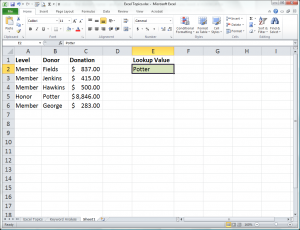
1. Enter a starting value in the field that is referenced by the VLOOKUP function. It should be a value near the top of the data list. In this case, Potter was entered.
2. Select the cell where the VLOOKUP formula will reside. In this example, that is cell F2.
3. In the Formula bar, type =VLOOKUP(
4. Complete the formula by entering each argument as described below. This helpful tool that shows you the full formula and its variables is called the Formula Autocomplete Tooltip. The components to the VLOOKUP formula and what they represent are detailed below.

• The lookup_value is the cell where the searched term is entered. In this example, cell E2 is where the donor's name is entered.
• The table_array should be the area of data that is searched for the lookup value and the returned value (in this case the donation amount). In this example, that is cells B2 (the top value-containing cell in the Donor column) through C18 (the bottom value-containing cell in the Donation column).
• The col_index_num is the number of the column in the selected array searched for the returned value. Column C is the one searched, and while it is Column three in your table (counting from left to right), it is only column two of the array you identified for the VLOOKUP. Two (for Column two) is entered here.
• The range_lookup value is either TRUE or FALSE. Entering a value of TRUE requires the searched column (the donor column in this example) to be in ascending order, and causes Excel to search for an approximate match. A selection of FALSE eliminates the ascending order requirement but searches only for an exact match. In this example, FALSE is selected.

1. Close the parentheses in the formula.
2. Press the ENTER key on your keyboard.
3. Review the result to check your work. =VLOOKUP(E2,B2:C18,2,FALSE)

Try this on your own data to build confidence with the function. Strengthening your overall Excel formulas skills will make VLOOKUP and related functions easier to apply in real-world scenarios. If you plan to apply your VLOOKUP formula to multiple cells, make sure your table arguments use absolute references.

Common VLOOKUP Errors and How to Fix Them

Even experienced Excel users run into VLOOKUP errors. Understanding what causes each error makes troubleshooting faster and less frustrating.

• #N/A error:The lookup_value is not found in the first column of the table_array. Check for typos, extra spaces or mismatched data types (for example, a number stored as text).

• #REF! error:The col_index_num exceeds the number of columns in the table_array. Reduce the column number or expand the range to include more columns.

• #VALUE! error: The col_index_num is less than 1 or is not a number. Ensure it is a positive integer — the same argument-validation principles apply to other Excel formulas like SUM.

• Wrong value returned:The range_lookup argument is set to TRUE (or omitted) and the first column is not sorted in ascending order. Set range_lookup to FALSE for an exact match.

• Partial match issues: Leading or trailing spaces in your data can cause mismatches even when values appear identical. Use the TRIM function to clean your data before running VLOOKUP.

VLOOKUP Best Practices

Following a few simple guidelines will help you avoid common mistakes and get reliable results from your VLOOKUP formulas.

• Always place the lookup_value in the first column of your table_array.

• Use FALSE for the range_lookup argument unless you specifically need an approximate match.

• Lock your table_array with absolute references (e.g., $B$2:$C$18) when copying the formula to other cells.

• Keep your data clean by removing duplicates, extra spaces and inconsistent formatting before running VLOOKUP.

• Use named ranges or formatted Excel Tables to make formulas easier to read and maintain.

• Test your formula with a known value first to confirm it returns the expected result.

VLOOKUP vs. XLOOKUP, INDEX/MATCH and HLOOKUP

VLOOKUP is a powerful function, but it is not always the best choice. Depending on your version of Excel and the structure of your data, one of these alternatives may be a better fit.

• XLOOKUP: A newer function available in Microsoft 365 and Excel for the web that can search in any direction, defaults to an exact match and includes built-in error handling. XLOOKUP is the recommended modern replacement for VLOOKUP when your version of Excel supports it.

• INDEX/MATCH: A combination of two functions that offers more flexibility than VLOOKUP. The lookup column does not need to be the first column in the range, and INDEX/MATCH handles large datasets more efficiently. This combination is preferred by advanced users who need greater control over their formulas.

• HLOOKUP: Works like VLOOKUP but searches horizontally across a row instead of vertically down a column. Use HLOOKUP when your data is organized in rows rather than columns.