How to Hide Formulas in Excel and Protect Your Spreadsheet

Excel makes it easy to decipher why a formula produces its result. When you click on the cell, the formula is displayed in the formula bar. If that’s not enough, you can select the Formulas ribbon and click Evaluate Formulas for a step-by-step walkthrough.

But what happens when you don’t want the formulas displayed? If you are working with a lot of complexity, it can get cluttered or confusing fast. Perhaps you need to hide Excel formulas from recipients and users for proprietary, security, or confidentiality reasons. On occasion I need to send the same spreadsheet to a list of competing vendors. I don’t want them to know how other producers’ rates are calculated.

Luckily, Excel makes it fairly simple to hide formulas. Just follow the steps below.

Unprotect the Sheet

1. On the Review ribbon, find the button labeled either Protect Sheet or Unprotect Sheet.
2. If the button is labeled Protect Sheet, then do nothing. The sheet is currently unprotected.
3. 
4. If the button is labeled Unprotect Sheet, then click it. The sheet is now unprotected.

Hide the Formulas

By default, when you click on a cell, its formula appears in the formula bar.

To hide formulas:

1. Select the cells for which you to want to hide the formulas.
2. Right-click the cell (or cells) and choose Format Cells.
3. In the Format Cells dialog box, click the Protection tab.
4. Check the Hidden box.
5. Note: Hidden is what prevents the user from seeing the formula. Locked prevents the user from changing the contents of the cell. Locked is set by default.
6. 
7. Click OK.

Protect the Sheet

Important Step: Setting the cell format to hidden has no effect until you protect the sheet!

1. On the Review ribbon, click Protect Sheet.
2. In the Protect Sheet dialog box, type a password. No one (including yourself) will be able to unprotect the sheet to make changes without typing the password, so do not forget the password!
3. 
4. Notice that by default the Select locked cells and Select unlocked cells checkboxes are selected. If you select OK now, the user without the password can do nothing but click on cells, whether those cells are locked or unlocked. S/he cannot format, delete, insert, or edit. If you want your users to do any of these operations for unlocked cells, then check them here.
5. Click OK.
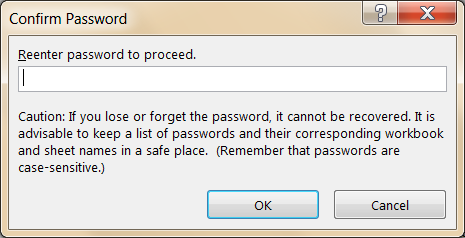
6. In the Confirm Password dialog box, Excel asks you to retype the password you selected. This prevents a typographical error in the password from locking up your spreadsheet forever. Retype the password and click OK.
7. 

That’s it! The formulas in your worksheet are now protected, and your users cannot see or edit the formulas. To verify it, click on a formula:

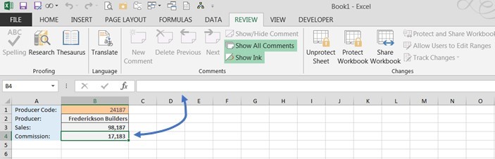
The formula no longer appears in the formula bar.

Next Steps

Try some of the other options to customize the protection properties, such as unlocking only specific input cells. This allows you to send a spreadsheet out to multiple users with an input cell—B1 in this example, where the user would enter his producer code—yet prevent the user from accessing other cells. This is a convenient tool for distributing corporate results to company agents, employees, or others while filtering the values so that each user can see only those for which he is authorized. For step by step instructions visit our blog post: How to Unlock Specific Cells in Excel.