What Does an Effective Employee Training Program Look Like?

As document sharing and co-authoring becomes the norm for how data is gathered and analyzed, it is more important than ever to make sure that there are guardrails in place for ensuring data quality. Variations in spelling, abbreviations, formatting and numerical styles can all radically impact results.

Let’s look at a simple example:

Your event planning company is preparing for a large company meeting. Managers from each department have been tasked with gathering and reporting meal orders, chosen from six meal options, into a shared event spreadsheet. This is the form you sent and the list of meal options offered:

Lunch Items

Grilled Chicken Sandwich

Cobb Salad

Hamburger

Chicken Salad

Veggie Burger

Fruit & Cheese Plate

And this is the PivotTable you generate after managers have entered the data:

SAVE $10 AND TRAIN ON THIS TOPIC TODAY

You’d hoped to get a quick count of the number of each meal you need to prepare. Instead, the way items have been recorded makes it very difficult to tally. Variations such as “chicken sandwich” and “grilled chicken sandwich” have been given their own line. Cobb Salad is misspelled at least once, also creating a separate entry. You would need to make additional calculations to know how many of an item to prepare in several cases.

And that’s if you can even figure out what people want. Some answers are so unclear, such as “chicken” (there are two chicken options) and “vegetarian” (there are two vegetarian options), that you have to go back to the managers for clarification. One cheeky attendee went completely off menu and ordered Pizza!

Finally, you notice that there are two rows for “Chicken” counted separately. Upon deeper inspection this happened because there are several hidden spaces after one of the entries, further muddying the data.

These data anomalies could have been avoided with a Drop-Down list. They are especially useful in forms and when your data is limited to a relatively small number of options. Here are three ways to add a drop-down list to your Excel spreadsheet:

Manually Type in Drop-Down List Items

Drop-down lists are created using the Data Validation tool. To begin, select the cell on your worksheet that is to display the list, then click the Data tab. Click the Data Validation button in the Data Tools group.

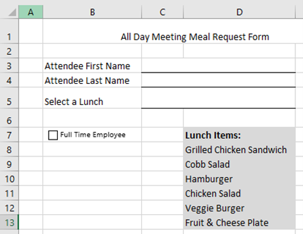
In the Data Validation dialog window, choose List from the Allow: dropdown menu on the Settings tab. Then, in the Source: field, type in each item of your list separated by a comma. In this example type: Grilled Chicken Sandwich, Cobb Salad, Hamburger, Chicken Salad, Veggie Burger, Fruit & Cheese Plate.

Click OK. The list will be applied to the cell and when the user clicks on the drop-down arrow, they can select an option to apply to the cell data.

If your list changes later, you will have to open the Data Validation dialog window and edit the text in the Source: field. Because the field is small, and even short lists can become difficult to edit in this way, the next method for applying a drop-down list is more common.

Create a Drop-Down List from Excel Cell Data

To use this method, you must first prepare the list you want included in the dropdown. Somewhere in your workbook, typically in a new worksheet, type the items you want included in your drop-down list. For this example, we have created a new tab called Menu Options and entered our six menu choices.

Now, return to the form worksheet and select the cell where the drop-down list goes.

Click the Data tab, then click the Data Validation button in the Data Tools group to open the Data Validation dialog window. Choose List from the Allow: dropdown menu on the Settings tab. Then, in the Source: field, enter the range where your list items are located. You can do this easily by simply clicking in the field, then clicking and dragging to select the items. Be sure NOT to include any headings that you don’t want offered as a selection option.

If your list changes later, simply change the data in the source cells. If you are adding or removing items, open the Data Validation dialog window and edit the list range in the Source: field to reflect the change in number of items.

If your list changes frequently, especially if the number of items changes frequently, you may want to consider creating a dynamic drop-down list for your form.

Create a Dynamic Drop-Down List from an Excel Table

The first step in preparing your list for a dynamic dropdown is the same as above: Somewhere in your workbook, type the items you want included in your drop-down list. Then, convert the list to a table by selecting any cell in the range and then hitting Ctrl+T. Next, give your table a more memorable name in the Table Name: field on the Table Design contextual tab.

Now, return to the form worksheet and select the cell where the drop-down list goes and open the Data Validation dialog window. In the Source: field enter the following formula where the arguments are the name you gave the table, “LunchMenu”, and the column heading within that table that should be used if more than one:

=INDIRECT(“LunchMenu[Menu]”)

While this is a more advanced technique and you need to remember the formula to execute it, you can now easily edit the table, adding or removing items without having to change the form or the Data Validation Source at all!

Data Validation is an extremely useful tool within the Excel user environment and drop-down lists are just one way to ensure that your data is consistent, accurate and – most importantly – useful! Give drop-down lists a try on your next collaborative form.

Learn More About Data Validation:

Automatically Stop Duplicate Values on Input

Excel Data Validation: Check Formatting of Entered Data

Tips for Data Management in Excel

Additional related Excel training courses available through Pryor Learning:

Microsoft® Excel® Forms & Reporting Made Easy

Advanced Microsoft Excel