No Excel Multiplication Formula? 3 Ways to Multiply in Excel

While there is no “Excel multiply formula” there are multiple ways to multiply in Excel. For instance, do you use an asterisk (*) to multiply, but hit a brick wall when you apply other arithmetic operators? What about shortcuts for multiplying many numbers in one step?

Read on for three powerful ways to perform an Excel multiply formula.

1. Multiplication with *

To write a formula that multiplies two numbers, use the asterisk (*). To multiply 2 times 8, for example, type “=2*8”.

Use the same format to multiply the numbers in two cells: “=A1*A2” multiplies the values in cells A1 and A2.

You can mix and match the * with other arithmetic operators, such as addition (+), subtraction (-), division (/), and exponentiation (^). In these cases, remember that Excel carries out the operations in the order of PEMDAS: parentheses first, followed by exponents, multiplication, division, addition, and subtraction.

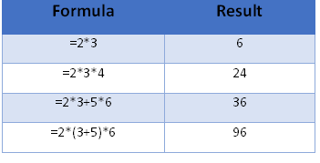In the following formula “=2*3+5*6,” Excel performs the two multiplication operations first, obtaining 6+30, and add the products to reach 36.

What if you want to add 3+5 before performing the multiplication? Use parentheses. Excel will always evaluate anything in parentheses before resuming the remaining calculations following PEMDAS. In the case of “=3*(3+5)*6”, Excel adds 3 and 5 first, resulting in 8. Then it multiplies 3*8*6 and reaches 144.

If you have trouble remembering the order of PEMDAS, use the Aunt Sally mnemonic device: use the first letters of the sentence, “Please Excuse My Dear Aunt Sally.”

2. Multiplication with the PRODUCT Function

When you need to multiply several numbers, you might appreciate the shortcut formula PRODUCT, which multiplies all of the numbers that you include in the parentheses.

The arguments can be:

Numbers or formulas separated by commas, such as:

=PRODUCT(3,5+2,8,3.14)

This is equivalent to =3*(5+2)*8*3.14.

Cell references separated by commas, such as:

=PRODUCT(A3,C3,D3,F3)

This is equivalent to =A3*C3*D3*F3.

A range of cells containing numbers, or multiple ranges separated by commas, such as:

=PRODUCT(F3:F25)

which is equivalent to =F3*F4*F5*(and so on, all the way up to)*F25, or:

=PRODUCT(F3:F25,H3:H25)

Any combination of numbers, formulas, cell references, and range references.

In each case, Excel multiplies all the numbers to find the product. If a cell in the range is empty or contains text, Excel leaves that cell’s value out of the calculation. If a cell in the range is zero, the product will be zero.

3. Multiplication of Ranges with the SUMPRODUCT Function

Consider the following invoice. The formula in Column E (with the formula shown to the right of the table) multiplies quantity by the price each to reach an extended price. The total in cell E7 sums up the extended prices.

But what if you don’t want the extended prices to show as separate calculations? What if you want to do it all in one step?

Try the SUMPRODUCT function, which multiplies the cells in two ranges and sums the results.

SUMPRODUCT(D2:D5,C2:C5) multiplies D2*C2, D3*C3, etc., and sums the results. Note that the result, 84.50, is the same as the previous example.

This function is invaluable for calculating weighted averages, such as classroom grades or prices based on variable state tax, in which you multiply a range of values by a range containing the weights.

Next Steps

These are but three of the methods to multiply numbers in Excel formulas. When you’ve mastered them, try the PRODUCTIF formula, which multiplies all numbers in a range if a condition is met.

Until then, try mixing and matching the multiplication formulas, using any combination along with other arithmetic functions, to create complex mathematical models.