Excel
May 4, 2026
Excel Formulas and Functions: A Guide to Syntax, Operators & Functions
Key Takeaways
- Every Excel formula begins with an equal sign (=) and uses a specific syntax of operators, cell references and parentheses to calculate results.
- Functions are prebuilt formulas (like SUM, AVERAGE and IF) that save time by packaging common calculations into a simple, reusable syntax.
- Excel follows the PEMDAS order of operations, so understanding operator precedence is essential to getting accurate results.
- Mastering a handful of core functions and best practices will help you work faster, reduce errors and build more powerful spreadsheets.
What Are Excel Formulas and Functions?
Excel makes it a simple task to perform mathematical operations. Using excel formula syntax, you can calculate and analyze data in your worksheet. Whether you're brand new to spreadsheets or looking to sharpen your skills, understanding excel formulas and functions is the foundation for everything you do in Excel.
As a reminder:
- Formulas are equations that combine values and cell references with operators to calculate a result.
- Functions are prebuilt formulas that can be quickly fed values without the need to write the underlying formula yourself.
Think of it this way: a formula is any calculation you build in a cell (for example, =A1+B1), while a function is a named shortcut that handles a specific calculation for you (for example, =SUM(A1:A10)). Both rely on the same underlying syntax rules, and once you understand those rules, you can read and write virtually any formula with confidence.
But to use either, you need to know how to write in their own language, which is commonly referred to as operators. And, like any language, operators have their own form of grammar, referred to as Order of Precedence.
Key Components of Excel Formula Syntax
Before diving into specific operators, it helps to understand the building blocks that make up every formula. Learning how to read excel formula syntax means recognizing these core components:
- Equal sign (=): Every formula starts here. The equal sign tells Excel that the characters that follow should be evaluated as a calculation, not displayed as plain text.
- Function name: A keyword like SUM, AVERAGE or IF that tells Excel which prebuilt calculation to run.
- Arguments: The values, cell references or ranges you provide inside parentheses for a function to work with. For example, in =SUM(A1:A10), the range A1:A10 is the argument.
- Parentheses: Group arguments together and control the order in which Excel evaluates parts of a formula.
- Comma separators: Separate multiple arguments within a function. In =IF(A1>10, "Yes", "No"), commas divide the condition from the true and false results.
- Cell references and ranges: Addresses like A1 or B2:B10 that point to specific cells or groups of cells. References can be relative or absolute (more on that later in this guide).
The Equal Sign
The equal sign is the gateway to every formula. Without it, Excel treats your entry as text or a static value. Type = and Excel immediately switches into calculation mode, ready to evaluate whatever comes next.
Function Names and Arguments
A function name like SUM or VLOOKUP tells Excel which prebuilt calculation to perform. The name is always followed by parentheses containing one or more arguments, which are the inputs the function needs. Arguments can be cell references, ranges, typed values or even other functions nested inside.
For example, in =AVERAGE(B2:B50), the function name is AVERAGE and the argument is the range B2:B50.
Cell References and Ranges
Cell references are how you point a formula to specific data in your worksheet. A single reference like A1 points to one cell, while a range like A1:A10 covers a block of cells. You can also reference cells on other sheets (Sheet2!A1) or in other workbooks.
References can be relative or absolute, which affects how they behave when you copy a formula. We cover this distinction in the Absolute vs. Relative Cell References section below.
Operators Used in Excel Formulas and Functions
Operators are the symbols that tell Excel what type of calculation or comparison to perform. Excel uses three main categories of operators.
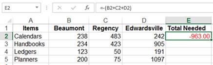
Mathematical Operators
To perform basic mathematical operations such as addition, subtraction or multiplication; to combine numbers; and to produce numeric results, use the following arithmetic operators.
Examples:
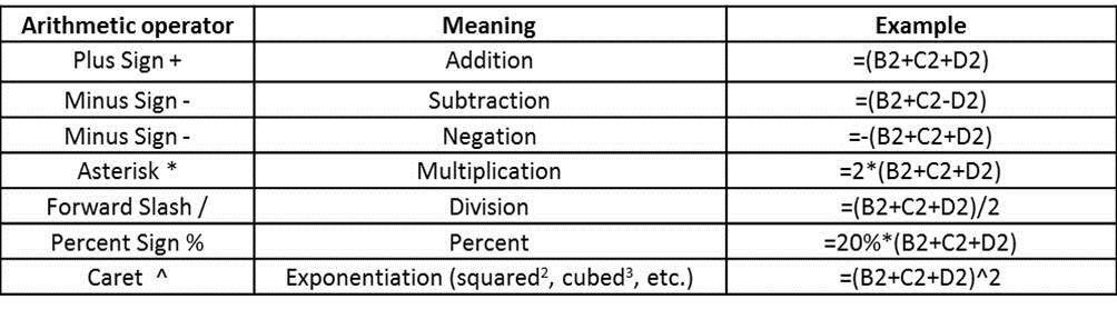
Comparison Operators
You can compare two values with the following operators. When two values are compared by using these operators, the result is a logical value, either TRUE or FALSE. These same operators power features like conditional formatting.
Example:
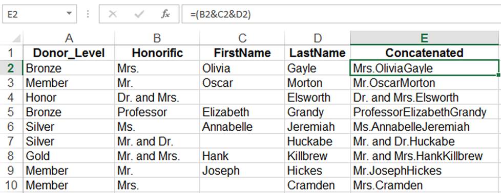
Text Concatenation Operator
Use the ampersand (&) to join, or concatenate, one or more text strings to produce a single piece of text.
Example:
Order of Precedence: How Excel Performs Operations
The order in which a calculation is performed affects the result, so it is important to understand how the order is determined and how you can change it to obtain desired results.
A formula in Excel always begins with an equal sign (=). The equal sign tells Excel that the succeeding characters are part of a formula or function. After the equal sign are the elements to be calculated (the operands), which are separated by calculation operators. Excel calculates from left to right, using the PEMDAS (Parentheses, Exponents, Multiplication, Division, Addition, Subtraction) order of operations.
In other words, it performs calculations in parentheses first, then it checks for multiplication and division, then finally it performs addition and subtraction. Using these rules of math is what makes it possible to do some potentially confusing problems that have many possible results if you do not follow the right order. Knowing that this is how Excel reads math, you need to structure your formulas accordingly.
2+3x4-5/6=?
If this problem were performed just from left to right, the answer would be 2.5. However, your intent might have been very different. Adding parentheses to show which items should be calculated first helps.
(2+(3x4)-5)/6
This same set of numbers with parentheses added calculate to a much different total. 3x4 is calculated first, for a total of 12. Then 2 is added to get 14, from which 5 is subtracted to get 9. Finally, 9 is divided by 6 for a total of 1.5.
Essential Excel Functions to Know
Now that you understand operators and the order of operations, you're ready to put that knowledge to work with some of the most widely used basic excel formulas. The table below summarizes seven essential functions you'll encounter in nearly every spreadsheet.
| Function | Syntax | What It Does | Example |
|---|---|---|---|
| SUM | =SUM(range) | Adds all values in a range | =SUM(B2:B50) |
| AVERAGE | =AVERAGE(range) | Returns the arithmetic mean | =AVERAGE(C2:C100) |
| COUNT | =COUNT(range) | Counts cells containing numbers | =COUNT(A1:A20) |
| COUNTA | =COUNTA(range) | Counts all non-empty cells | =COUNTA(A1:A20) |
| MAX / MIN | =MAX(range) / =MIN(range) | Returns the largest or smallest value | =MAX(D2:D30) |
| IF | =IF(condition, value_if_true, value_if_false) | Tests a condition and returns one of two results | =IF(A1>100, "Over", "Under") |
| VLOOKUP | =VLOOKUP(lookup_value, table_array, col_index, [range_lookup]) | Searches the first column of a range and returns a value from a specified column | =VLOOKUP("Widget", A2:D50, 3, FALSE) |
SUM
=SUM(range) is the most-used function in Excel. It adds every numeric value in the range you specify. Instead of writing =A1+A2+A3+A4, you can simply write =SUM(A1:A4) and get the same result with far less effort.
AVERAGE
=AVERAGE(range) returns the arithmetic mean of the values in a range. It's the go-to function for finding typical values in a dataset, such as average sales per month or average test scores.
COUNT and COUNTA
=COUNT(range) counts only cells that contain numbers, while =COUNTA(range) counts all non-empty cells regardless of data type. Use COUNT when you need to know how many numeric entries exist and COUNTA when you want to count any cell that isn't blank.
MAX and MIN
=MAX(range) returns the largest value in a range and =MIN(range) returns the smallest. These functions are useful for quickly identifying highs and lows, such as the highest invoice amount or the lowest temperature reading in a dataset.
IF
=IF(condition, value_if_true, value_if_false) introduces logical testing to your spreadsheets. You provide a condition (like A1>100), and Excel returns one result when the condition is true and a different result when it's false. IF is the foundation for decision-making logic in Excel and can be nested for more complex scenarios.
VLOOKUP
=VLOOKUP(lookup_value, table_array, col_index, [range_lookup]) searches for a value in the first column of a table and returns a corresponding value from another column. It's one of the most powerful lookup functions in Excel and is commonly used to pull data from reference tables. Set the last argument to FALSE for an exact match.
CONCATENATE (CONCAT)
=CONCATENATE(text1, text2, ...) or the newer =CONCAT(text1, text2, ...) joins multiple text strings into one. For example, =CONCAT(A1, " ", B1) combines a first name and last name with a space between them. You can also use the & operator covered in the Text Concatenation Operator section above to achieve the same result.
Absolute vs. Relative Cell References
One of the most common sources of formula errors happens when you copy a formula to a new cell and the results suddenly look wrong. The reason usually comes down to cell references.
- Relative reference (A1): Adjusts automatically when you copy a formula. If you write =A1*B1 in row 1 and copy it down to row 2, Excel changes it to =A2*B2. This is the default behavior and is useful when you want the same calculation applied across multiple rows or columns.
- Absolute reference ($A$1): Stays locked to a specific cell no matter where you copy the formula. The dollar signs tell Excel not to adjust the reference. Use this when a formula needs to always point to the same cell, such as a tax rate stored in one location.
- Mixed reference ($A1 or A$1): Locks either the column or the row but not both. $A1 keeps the column fixed while allowing the row to change. A$1 keeps the row fixed while allowing the column to change.
For example, imagine you have a price in column B and a single tax rate in cell E1—a common scenario in Excel finance formulas. Your formula in C2 might be =B2*$E$1. When you copy this formula down the column, B2 adjusts to B3, B4 and so on (relative), but $E$1 stays locked (absolute), ensuring every row uses the same tax rate.
Formula Tips and Best Practices
Knowing the syntax is only half the battle. These practical tips will help you write cleaner formulas and avoid common mistakes:
- Use cell references instead of hardcoded numbers. Typing =A1*0.08 works, but storing the rate in a cell and referencing it (=A1*$B$1) makes your spreadsheet easier to update and audit.
- Break complex formulas into smaller steps. If a formula is getting long and hard to read, split it across helper cells. You can always hide those columns later.
- Use named ranges for readability. Instead of =SUM(B2:B500), define the range as "MonthlySales" and write =SUM(MonthlySales). It's easier to understand at a glance.
- Double-check with formula auditing tools. Excel's Trace Precedents and Evaluate Formula features (found on the Formulas tab) let you see exactly which cells feed into a formula and how Excel evaluates it step by step.
- Test formulas with known values. Before applying a formula to a large dataset, test it on a few rows where you can manually verify the result.
- Add comments or notes to document complex formulas. Right-click a cell and choose "Insert Comment" or "New Note" to explain what a formula does. Your future self (and your coworkers) will thank you.
Build Your Excel Skills with Pryor Learning
Now that you have the foundation of excel formula syntax, from operators and the order of operations to essential functions and best practices, you're well on your way to building more powerful and accurate spreadsheets. Like any skill, formula writing improves with practice and continued learning.
Pryor Learning offers a range of Excel training courses designed for every skill level, from beginners learning their first SUM function to advanced users tackling complex data analysis. Choose from live seminars, On-Demand courses and the PryorPlus subscription for unlimited access to hundreds of professional development topics.


