Excel, Macros
Mar 12, 2013
Excel Array Formulas: A Practical Guide with Examples
Key Takeaways
Array formulas let you perform calculations across multiple cells or ranges at once, enabling multi-criteria logic that standard functions cannot handle alone.
Legacy array formulas require Ctrl + Shift + Enter to activate, and Excel confirms them by wrapping the formula in curly braces.
Modern versions of Excel support dynamic array formulas that spill results automatically, reducing the need for CSE entry.
Common errors like #VALUE and #SPILL are easy to fix once you understand how array formulas process data.
What Are Excel Array Formulas?
An array is simply a range of values, whether that range is a column, a row or a block of cells. Excel array formulas are formulas that operate on an entire range of values rather than a single cell. Instead of calculating one value at a time, an array formula processes multiple values simultaneously and can return one result or many.
Regular formulas work cell by cell. If you write a SUM formula, it adds up the values you specify. An array formula goes further by letting you embed conditions, multiply ranges together and perform calculations that would otherwise require helper columns or multiple formulas working in tandem.
Single-Cell vs. Multi-Cell Array Formulas
A single-cell array formula returns one result from a calculation that spans an entire range. The multi-criteria SUM example later in this article is a single-cell array formula: it evaluates dozens of rows but produces a single total. A multi-cell array formula, by contrast, returns results across multiple cells. For example, you could use a multi-cell array formula to multiply every value in one column by a corresponding value in another column and display all the products at once.
When to Use Array Formulas
Array formulas are especially useful when standard functions fall short. Common scenarios include:
Multi-criteria summing or counting: Add or count values that meet two or more conditions at the same time, such as totaling sales for a specific product in a specific region.
Comparing two ranges: Check whether every value in one list appears in another without writing a formula for each row.
Conditional aggregation: Calculate averages, minimums or maximums based on multiple criteria.
Replacing helper columns: Perform intermediate calculations inside a single formula instead of dedicating extra columns to them.
Creating calculated arrays for charts: Generate a derived data set on the fly for use in an Excel chart or report.
When a single IF or SUM function is not enough to capture the logic you need, an array formula is often the answer.
How to Enter an Array Formula in Excel
Legacy array formulas use a special entry method. After typing the formula, press Ctrl + Shift + Enter instead of the standard Enter key. Excel confirms the entry by wrapping the formula in curly braces {} in the formula bar. These braces are added automatically; typing them yourself will not work and will cause an error.
In Microsoft 365 and recent versions of Excel that support dynamic arrays, many array-capable functions accept a standard Enter keystroke and produce results that "spill" across adjacent cells. However, if you are using an older version of Excel or writing a legacy SUM-based array formula like the one in the walkthrough below, Ctrl + Shift + Enter is still required.
Array Formula Walkthrough: Multi-Criteria SUM
To see how array formulas solve problems that standard functions cannot, consider the following scenario. You may be familiar with the IF function in Excel, which lets a cell display one of two possible values, depending on whether a condition is true or false. The syntax is:
=IF(condition to test, value if the condition is true, value if the condition is false)
Note that whenever a function has multiple arguments, you separate them with commas.
For example, let's say if the value of B5 is less than 100, you want B6 to have a value of 6%, and if B5 has a value that's 100 or higher, you want B6 to have a value of 8%. You would enter this into B6:
=IF(B5<100,6%,8%)
That's a great feature, but what if you want to test for two conditions? For example, let's say you're selling different types of fruit to customers in multiple states, and you want to add only the sales of apples to New Jersey, but not apples to New York, or bananas to New Jersey. The IF function can't do that, but an Excel array formula can.
With an array formula, rather than calculating values of individual cells, you calculate the values of multiple cells (a range) at once. What's also different about array formulas is that you must enter them by pressing Ctrl + Shift + Enter, rather than just the Enter key, by itself.
Here is a list of orders we received. We'll put the array formula in D17.
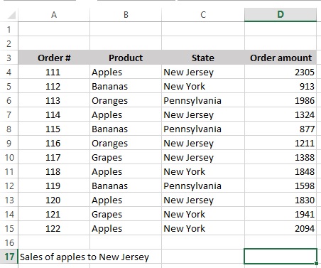
Type this into D17 (not case-sensitive):
=SUM((D4:D15)*(B4:B15="apples")*(C4:C15="new jersey"))
This formula tells Excel to use the SUM function on column D, but only in the rows where columns B and C meet your criteria for fruit and state. Since the criteria are text and not numbers, you need to put them in quotes.
After typing the formula, make sure to press Ctrl + Shift + Enter as described above, or Excel will throw a #VALUE error.
The result in D17 should be 5459, since it doesn't include order #118 or #122, which are for different states. Also look at the formula bar:

Excel appended curly braces to the beginning and end. That's how you know it's an array formula. If you're a good typist, resist the temptation to type the braces yourself. It won't work.
Think you got it? On your own, go to D18 and calculate the sales of bananas to Pennsylvania. Download multiple Array Formula 1_criteria.xlsx for a head start.
Legacy Array Formulas vs. Dynamic Array Formulas
Excel has evolved significantly since legacy array formulas were introduced. The walkthrough above demonstrates a CSE (Ctrl + Shift + Enter) array formula, which is the traditional method. These formulas still work in every version of Excel, but Microsoft 365 and Excel for the web now support dynamic array formulas that behave differently.
Dynamic array formulas "spill" their results automatically. When a formula returns multiple values, Excel fills adjacent cells with those results without requiring you to select a range in advance or press Ctrl + Shift + Enter. A single formula entered in one cell can populate an entire column or block of cells. The spill range operator (#) lets other formulas reference the full set of spilled results.
This means many tasks that once required CSE array formulas can now be handled more simply with dynamic array functions. Legacy CSE formulas remain fully supported, so existing workbooks will continue to function. However, if you are working in Microsoft 365, dynamic arrays are generally the more efficient approach for new formulas.
Key Dynamic Array Functions
FILTER: Returns rows from a range that meet one or more criteria you specify.
SORT: Sorts a range or array by one or more columns in ascending or descending order.
SORTBY: Sorts a range based on values in a corresponding range, giving you more flexible sorting logic.
UNIQUE: Extracts distinct values from a range, removing duplicates automatically.
SEQUENCE: Generates a series of sequential numbers in a row, column or grid.
RANDARRAY: Creates an array of random numbers with dimensions and bounds you define.
Common Array Formula Errors and How to Fix Them
Array formulas can produce confusing errors if the entry method or cell setup is not quite right. Here are the most common issues and how to resolve them:
#VALUE error: This typically means you pressed Enter instead of Ctrl + Shift + Enter when entering a legacy array formula. Select the cell, press F2 to edit and then press Ctrl + Shift + Enter to confirm the formula as an array.
#SPILL error: This occurs with dynamic array formulas when the spill range is blocked by existing data in one or more cells. Clear the obstructing cells so the formula has room to display all its results.
#REF error: Mismatched array dimensions can trigger this error. If your formula references two ranges that have different numbers of rows or columns, Excel cannot align them. Make sure all ranges in the formula are the same size.
Circular references: If an array formula references a cell within its own output range, Excel will flag a circular reference. Move the formula to a cell outside the range it calculates.
Strengthen Your Excel Skills with Pryor Learning
Array formulas are just one of the many powerful features that can transform how you work in Excel. Pryor Learning offers live instructor-led seminars and on-demand courses covering Excel array formulas, dynamic arrays, advanced functions and more. Whether you are building your first array formula or looking to master advanced Excel capabilities including dynamic arrays, Pryor's training programs meet you at your level. Explore PryorPlus for unlimited access to hundreds of courses that sharpen your skills and advance your career.