Excel, VLOOKUP
May 8, 2026
How to Use VLOOKUP in Excel: A Step-by-Step Example for Merging Tables
Key Takeaways
- VLOOKUP searches for a value in the first column of a range and returns a corresponding value from another column, making it ideal for merging data from separate tables.
- The VLOOKUP formula requires four arguments: lookup_value, table_array, col_index_num and range_lookup (exact match or approximate match).
- You can use a single VLOOKUP formula to combine two tables in Excel, such as pulling department data from a Payroll list into an HR list, then copy the formula down to fill all rows.
- Common VLOOKUP errors like #N/A error usually result from mismatched data types, extra spaces or an incorrect table range.
What Is VLOOKUP?
VLOOKUP (Vertical Lookup) ranks among the most useful Excel lookup functions for pulling data from multiple column-sorted lists into a unified table. It searches the leftmost column of a specified range for a lookup value and returns data from the same row in a different column. Think of it this way: the function asks a simple question and returns the answer. Question: is the data from a specific cell reference in this column? If so, give me the corresponding value from another column.
HLOOKUP (Horizontal Lookup) works the same way but searches across a row instead of down a column. For most table-merging tasks, VLOOKUP is the go-to function because users typically organize spreadsheet data in columns.
VLOOKUP Syntax and Arguments
The generic VLOOKUP formula looks like this:
=VLOOKUP(lookup_value, table_array, col_index_num, [range_lookup])
Here is what each argument means:
| Argument | Description | Example Value |
|---|---|---|
| lookup_value | The value you want to find in the first column of the range | 18648 |
| table_array | The range of cells containing the data you want to search | G2:H6 |
| col_index_num | The column number in the range from which to return a value (counting from the left) | 2 |
| range_lookup | FALSE (or 0) for an exact match; TRUE (or 1) for an approximate match | FALSE |
- lookup_value is the key that connects your two tables, such as an Employee ID.
- table_array is the range where VLOOKUP will search. The lookup value must be in the first column of this range.
- col_index_num tells VLOOKUP how many columns over to find the data you want returned.
- range_lookup determines match type. Use FALSE for an exact match in most cases. Use TRUE only when working with sorted data and you need the closest value.
VLOOKUP Example: Merging an HR List and a Payroll List
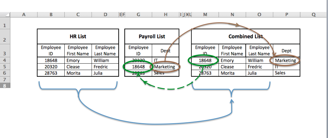
Let's use VLOOKUP to pull information from two lists, HR and Payroll, to create a Combined List. The HR List contains Employee ID, Employee First Name and Employee Last Name. The Payroll List contains Employee ID and Dept. Our goal is to merge these tables so the Combined List has the headings: "Employee ID," "Employee First Name," "Employee Last Name" and "Dept."
Step-by-Step: Using VLOOKUP to Combine Two Tables
1) We'll start by copying and pasting the HR List into the Combined List and entering "Dept" into the next column heading in the Combined List. Now we'll fill in the Employee's Dept using VLOOKUP.
The VLOOKUP function needs:
- a value to match
- a location to search
- the number of columns over to the data we want
- whether an exact match is needed or not
2) Locate the Employee ID 18648 in the Combined List.
3) Next, we'll locate the "Employee ID" and "Dept" headings in the Payroll List cells (G2:H6) and count the columns from "Employee ID" to "Dept" to get the column_index 2.
4) Scan that many places along 18648's row to select "Marketing."
5) To enter "Marketing" as 18648's Dept we'll set that cell value equal to the result of this VLOOKUP formula:
=VLOOKUP(18648,G2:H6,2,FALSE)
NOTE: The last argument should be FALSE (or 0) for an exact match to the Employee ID, or TRUE (or 1) for an approximate match. Approximate match requires you to sort the lookup column in ascending order. (See the Excel documentation for a detailed explanation.)
6) Now, select the cell with the VLOOKUP formula, then drag the fill handle (the small square at the bottom-right corner of the cell) down through all remaining rows in the Dept column, and you're done!
Common VLOOKUP Errors and How to Fix Them
Even a well-constructed VLOOKUP formula can return an error if you don't set up the data correctly. Here are the most frequent issues and how to resolve them:
- #N/A error — This means VLOOKUP could not find the lookup value in the first column of your table array. Common causes include extra spaces in cells, mismatched data types (for example, one table stores an Employee ID as text while another stores it as a number) or a misspelled value. Use the TRIM function to remove extra spaces and double-check that both columns use the same format.
- #REF! error — You see this error when the col_index_num is larger than the number of columns in your table_array. For example, if your range is only two columns wide but you enter 3 as the column index, Excel has nowhere to look. Reduce the col_index_num or expand the table_array range.
- #VALUE! error — You see this error when the col_index_num is less than 1. Make sure the column index is a positive whole number.
To prevent errors from disrupting your spreadsheet, wrap your VLOOKUP in an IFERROR function. For example:
=IFERROR(VLOOKUP(18648,G2:H6,2,FALSE),"Not Found")
This returns "Not Found" instead of an error code, keeping your Combined List clean and readable. You can also apply conditional formatting to highlight any cells that return "Not Found," making them easy to spot at a glance.
VLOOKUP vs. XLOOKUP: When to Use Each
If you're using Excel 365 or Excel 2021 and later, you have access to XLOOKUP, a more flexible successor to VLOOKUP. Key advantages of XLOOKUP include:
- It can search in any direction, including to the left, which VLOOKUP cannot do.
- It doesn't require a column index number. Instead, you specify a return array directly.
- It defaults to an exact match, so you don't need to remember to add FALSE.
- It supports dynamic arrays and can return multiple values at once.
VLOOKUP remains the better choice when you need backward compatibility with Excel 2019 or earlier, or when you're collaborating with colleagues who may not have access to XLOOKUP.
Another powerful alternative is INDEX/MATCH. This combination works in all Excel versions, can look in any direction and offers more flexibility than VLOOKUP. However, the syntax is slightly more complex—an advanced Excel skill—which is why many users prefer VLOOKUP for straightforward lookups.
Build Your Excel Skills with Pryor Learning
This may seem like a lot of steps to merge just two small files, but when you have multiple files and thousands of values, the initial effort to automate the process will be well worth your time and labor. Mastering functions like VLOOKUP, XLOOKUP and INDEX/MATCH is one of the fastest ways to boost your productivity in Excel.
Pryor Learning offers live virtual and In-Person Excel seminars as well as On-Demand courses covering VLOOKUP, XLOOKUP, pivot tables and more. With a PryorPlus subscription, you get unlimited access to hundreds of courses that sharpen your skills at every level.


