Automatically Stop Duplicate Values on Input in Excel

Key Takeaways:

You can prevent duplicates in Excel by combining Data Validation with the COUNTIF function.
The COUNTIF formula checks whether a value already exists in your selected range and blocks re-entry if it does.
Using the correct mix of absolute and relative references in the formula is essential for it to work.
You can customize both the input message and error alert users see when a duplicate is attempted.

You can prevent duplicates in Excel by setting up a Data Validation rule that uses the COUNTIF function to check for repeated entries automatically. This approach protects data integrity, keeps your spreadsheets cleaner and eliminates the need for tedious manual checks. The walkthrough below shows you exactly how to set it up step by step. This method works in Excel 2016, 2019, 2021 and Microsoft 365.

Step-by-Step Guide to Preventing Duplicate Entries in Excel

Follow these steps to create a Data Validation rule that blocks Excel duplicate data entry across a range of cells.

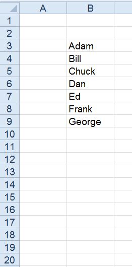
One) Select the range of cells where you want to prevent duplicate values (in this example, B3:B20). .

2) In Excel, on the Data tab, click Data Validation.

3) Once in the Data Validation dialog box, under the Settings tab click the Allow dropdown and select Custom from the list. A Formula field will appear.

4) In the Formula field type =COUNTIF($B$3:$B$20,B3)<2. When data is entered into a cell, this formula is evaluated. It looks for duplicate values.

See the sections below for a detailed breakdown of how this formula works and why the reference types matter.

Understanding the COUNTIF Formula

The formula =COUNTIF($B$3:$B$20,B3)<2 is the engine behind the duplicate prevention rule. Here is what each part does:

$B$3:$B$20 - The range Excel searches through. The dollar signs make this an absolute reference so the range stays fixed for every cell in the validation rule.
B3 - The criteria argument. This is a relative reference to the active cell, so Excel checks the value in whichever row the user is currently entering data.
<2 - The condition. If the COUNTIF function finds the value fewer than two times in the range, the entry is allowed. A count of two or more means a duplicate exists and the entry is rejected.

In plain language, the formula asks: "Does this value already appear in my list?" If the answer is yes, Excel blocks the entry.

Absolute vs. Relative References Explained

Getting the references right is the most common stumbling point when setting up this rule. Here is a quick comparison:

	Absolute Reference	Relative Reference
Syntax	$B$3:$B$20	B3
Behavior	Stays locked on the same range no matter which cell is active	Adjusts automatically to match the current row
When to Use	For the validation range so every cell checks against the full list	For the active cell argument so each row evaluates its own value

Absolute references are required for the range ($B$3:$B$20) because you want every cell in the validated area to compare against the entire list, not a shifting subset. The active cell reference (B3) must remain relative so it updates per row. If you accidentally lock both references, the formula will only ever check the value in B3 and the rule will not work correctly.

Customizing Input and Error Messages

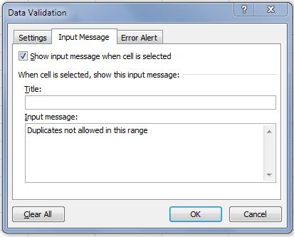
5) In the Data Validation dialog, click the Input Message tab and, if desired, type a message that will be displayed when the user selects a cell within the range of the Data Validation rule. Otherwise, if you don't want a message to appear every time someone selects a cell in the range, clear the 'Show input message...' option.

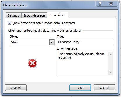
6) Click the Error Alert tab and type the message that will be displayed if the user enters a duplicate value in the range. Under the Style dropdown you will see three options: Stop, Warning and Information. Select Stop if you want to fully block duplicate entries. The Warning and Information styles display a message but still allow the user to override and enter the duplicate.

Best practices for writing clear error alert messages:

Keep the message short and specific (e.g., "This value already exists in the list. Please enter a unique value.")
Tell the user what to do next, not just what went wrong.
Use a descriptive title in the Title field so the alert is easy to identify.

7) Click OK.

Now test your Data Validation rule by entering values, including some duplicates, within the range.

Practical Tips for Preventing Duplicate Data in Excel

This technique is useful any time a column must contain only unique values. Common workplace use cases include:

Employee IDs or badge numbers
Invoice or purchase order numbers
Product SKUs
Email addresses in a mailing list
Customer account numbers

Once your rule is in place, keep these tips in mind:

Test immediately after setup. Enter a value, then try entering it again to confirm the error alert appears.
Expand the range as your list grows. If you expect more rows of data, set the validation range larger than your current list (e.g., $B$3:$B$500) so new entries are still checked.
Combine with Conditional Formatting. Apply a Duplicate Values highlight rule (Home > Conditional Formatting > Highlight Cells Rules > Duplicate Values) so existing duplicates are visually flagged alongside the prevention rule.
Use the Remove Duplicates tool for cleanup. If duplicates already exist in your data, go to Data > Remove Duplicates to delete repeated rows before applying the validation rule.
Double-check your references if the rule isn't working. The most common cause of failure is using relative references for the range or absolute references for the active cell.

Pryor Learning offers Excel training courses that cover Data Validation, formulas and other productivity techniques in depth. Whether you are building your first spreadsheet or streamlining complex workflows, structured training can help you get more from Excel faster.

Commonly Asked Questions

You can prevent duplicate entries in a single column by applying a Data Validation rule that uses the COUNTIF function to check whether a value already exists in the range. Select the column, open Data Validation, choose Custom and enter the formula =COUNTIF($B$2:$B$100,B2)<2, adjusting the range to match your column. Any repeated value will be blocked automatically.

Yes, you can remove the restriction by selecting the validated range, going to Data > Data Validation and clicking "Clear All." This removes the rule without affecting the data already entered. You can also edit the rule to change the formula or expand the range without starting over.

Yes, Excel has a built-in Remove Duplicates tool found on the Data tab that scans selected columns and deletes duplicate rows in one click. This is useful for cleaning up existing data, while Data Validation is better for preventing duplicates going forward.

You can highlight duplicates using Conditional Formatting by selecting your range, clicking Home > Conditional Formatting > Highlight Cells Rules > Duplicate Values and choosing a formatting style. This visually flags duplicates but does not block them from being entered. Pairing this with a Data Validation rule gives you both visual identification and active prevention.

Absolute references (like $B$3:$B$20) lock the range so it stays the same for every cell in your validation rule, while the relative reference (like B3) adjusts for each row so Excel checks the correct cell. Using the wrong reference type is the most common reason the duplicate prevention formula fails. Always use absolute references for the range and a relative reference for the active cell.