Excel
Apr 14, 2026
How to Multiply in Excel: 3 Methods with Formula Examples
Key Takeaways
- Use the asterisk (*) operator to multiply numbers or cells (e.g., =A1*B1) for quick, everyday calculations.
- Use the PRODUCT function to multiply large sets of numbers, cell references or ranges in a single formula.
- Use the SUMPRODUCT function to multiply corresponding values across two ranges and sum the results in one step.
- Excel has no dedicated MULTIPLY function, but these three methods cover every Excel multiplication formula scenario you'll encounter.
The Quick Answer: How to Multiply in Excel
The simplest way to multiply in Excel is to use the asterisk operator. For example, typing =A1*B1 into a cell multiplies the values in cells A1 and B1. If you need to multiply many values at once, the PRODUCT function handles that in a single formula. And when you need to multiply two ranges and add the results together, the SUMPRODUCT function does it all in one step.
Here's a quick comparison of the three methods:
| Method | Syntax Example | Best For |
|---|---|---|
| Asterisk (*) | =A1*B1 | Multiplying two or a few numbers or cells |
| PRODUCT | =PRODUCT(A1:A10) | Multiplying many cells or large ranges |
| SUMPRODUCT | =SUMPRODUCT(A1:A10,B1:B10) | Multiplying two ranges and summing the results |
While there is no dedicated "multiply" function in Excel, these three approaches cover everything from basic arithmetic to complex calculations. Read on for step-by-step instructions on each method.
How to Multiply in Excel Using the Asterisk (*)
To write a formula that multiplies two numbers, use the asterisk (*). To multiply 2 times 8, for example, type “=2*8”.
Use the same format to multiply the numbers in two cells: “=A1*A2” multiplies the values in cells A1 and A2.
You can mix and match the * with other arithmetic operators, such as addition (+), subtraction (-), division (/), and exponentiation (^). In these cases, remember that Excel carries out the operations in the order of PEMDAS: parentheses first, followed by exponents, multiplication, division, addition and subtraction.
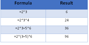
In the following formula “=2*3+5*6,” Excel performs the two multiplication operations first, obtaining 6+30, and add the products to reach 36.
What if you want to add 3+5 before performing the multiplication? Use parentheses. Excel will always evaluate anything in parentheses before resuming the remaining calculations following PEMDAS. In the case of “=3*(3+5)*6”, Excel adds 3 and 5 first, resulting in 8. Then it multiplies 3*8*6 and reaches 144.
If you have trouble remembering the order of PEMDAS, use the Aunt Sally mnemonic device: use the first letters of the sentence, “Please Excuse My Dear Aunt Sally.”An easy way to remember the order of PEMDAS is the mnemonic "Please Excuse My Dear Aunt Sally," where each word's first letter matches a step: Parentheses, Exponents, Multiplication, Division, Addition, Subtraction.
How to Multiply in Excel Using the PRODUCT Function
When you need to multiply several numbers, you might appreciate the shortcut formula PRODUCT, which multiplies all of the numbers that you include in the parentheses. PRODUCT is the closest thing Excel has to a dedicated multiply function, so if you've been searching for one, this is it.
The arguments can be:
- Numbers or formulas separated by commas, such as:
=PRODUCT(3,5+2,8,3.14)
This is equivalent to =3*(5+2)*8*3.14.
- Cell references separated by commas, such as:
=PRODUCT(A3,C3,D3,F3)
This is equivalent to =A3*C3*D3*F3.
- A range of cells containing numbers, or multiple ranges separated by commas, such as:
=PRODUCT(F3:F25)
which is equivalent to =F3*F4*F5*(and so on, all the way up to)*F25, or:
=PRODUCT(F3:F25,H3:H25)
- Any combination of numbers, formulas, cell references, and range references.
In each case, Excel multiplies all the numbers to find the product. If a cell in the range is empty or contains text, Excel leaves that cell’s value out of the calculation. If a cell in the range is zero, the product will be zero.
How to Multiply and Sum in Excel Using SUMPRODUCT
The SUMPRODUCT function multiplies corresponding values in two or more ranges and then adds the results, all in a single formula. Consider the following invoice. The formula in Column E (with the formula shown to the right of the table) multiplies quantity by the price each to reach an extended price. The total in cell E7 sums up the extended prices.

But what if you don’t want the extended prices to show as separate calculations? What if you want to do it all in one step?
Try the SUMPRODUCT function, which multiplies the cells in two ranges and sums the results.

SUMPRODUCT(D2:D5,C2:C5) multiplies D2*C2, D3*C3, etc., and sums the results. Note that the result, 84.50, is the same as the previous example.
This function is invaluable for calculating weighted averages, such as classroom grades or prices based on variable state tax, in which you multiply a range of values by a range containing the weights.
How to Multiply a Column by a Number in Excel
One of the most common tasks in Excel is multiplying every value in a column by the same constant. For example, you might need to apply a 10% price increase across an entire product list.
The formula approach uses an absolute reference to lock the constant in place. If your values are in column A and your multiplier is in cell B1, enter =A1*$B$1 in the adjacent cell. The dollar signs ensure B1 stays fixed when you copy the formula down the column.
You can also multiply columns in Excel without writing a formula at all using Paste Special:
- Type your multiplier (e.g., 1.10 for a 10% increase) into a blank cell and copy it.
- Select the range of values you want to multiply.
- Right-click, choose Paste Special, select Multiply and click OK.
Excel overwrites each selected cell with the multiplied result. This method is especially useful when you want to change values in place rather than create a separate output column. To visually flag results that exceed a threshold after multiplying, apply conditional formatting based on the updated values.
How to Multiply by a Percentage in Excel
You can multiply by a percentage in Excel using either the percentage symbol or its decimal equivalent. Both approaches produce the same result.
To calculate 15% of a value in cell A1, enter =A1*15% or =A1*0.15. Excel treats the percentage symbol as a division by 100, so 15% and 0.15 are identical internally.
If your percentage is stored in another cell (say B1, formatted as a percentage), simply use =A1*B1. Excel automatically reads the cell's underlying decimal value. This makes it easy to apply tax rates, discount percentages or commission rates across a range of figures—the same arithmetic that underpins many Excel finance formulas.
Troubleshooting: Why Your Multiplication Formula Isn't Working
If your multiplication formula displays the formula text instead of a result, or returns an unexpected value, check these common causes:
- Show Formulas mode is on. Excel has a toggle that displays raw formulas instead of calculated results. Press Ctrl + ` (the backtick key, usually above Tab) to switch back to normal view.
- Cells are formatted as text. When a cell is formatted as text, Excel treats its contents as a string rather than a number. Select the problem cells, change the format to Number or General then click into the formula bar and press Enter to force Excel to recalculate.
- Extra spaces or hidden characters. If you pasted data from another source, cells may contain invisible spaces or special characters that prevent Excel from recognizing the value as a number. Use the TRIM function (e.g., =TRIM(A1)) or the CLEAN function to strip out unwanted characters before multiplying.
If none of these fixes resolve the issue, check for circular references by going to Formulas > Error Checking > Circular References.
Next Steps
These are but three of the methods to multiply numbers in Excel formulas. When you've mastered them, try combining SUMPRODUCT with conditional logic or helper columns to multiply values only when specific criteria are met.
Mix and match the multiplication formulas, using any combination along with other arithmetic functions to build the kind of advanced Excel models that power real-world analysis. If you want to build your skills further, explore Pryor Learning's Excel formulas training for hands-on practice with functions and real-world scenarios.


