Excel, Formulas
May 1, 2026
How to Use the PMT Function in Excel (Plus FV, PV and NPER)
Key Takeaways
- The PMT function in Excel calculates the periodic payment required to pay off a loan or reach an investment goal based on a constant interest rate and a fixed number of periods.
- PMT is one of four core Excel finance formulas (along with FV, PV and NPER) that work together to solve time-value-of-money problems.
- Always divide the annual interest rate by 12 when calculating monthly payments and use a negative sign on the present value to return a positive payment amount.
- You can download the practice spreadsheet included in this guide to follow along and test your own numbers.
What Is the PMT Function in Excel?
The PMT function in Excel calculates the fixed periodic payment needed to pay off a loan or reach a savings goal. Whether you need a monthly payment on a mortgage, a loan repayment schedule or an annuity payment amount, the Excel PMT formula handles it all with a single function.
The syntax is:
=PMT(rate, nper, pv, [fv], [type])
Here is what each argument means:
| Argument | Description | Required? |
|---|---|---|
| rate | The interest rate per period. For monthly payments, divide the annual rate by 12. | Yes |
| nper | The total number of payment periods (e.g., 360 for a 30-year monthly mortgage). | Yes |
| pv | The present value, or total amount the loan or investment is worth today. | Yes |
| fv | The future value you want after the last payment. Defaults to 0 if omitted. | No |
| type | When payments are due: 0 (end of period, the default) or 1 (beginning of period). | No |
PMT is part of a family of related financial functions in Excel that share many of the same arguments. This guide walks you through PMT along with three other essential functions: FV, PV and NPER. Together they cover the most common time-value-of-money calculations you will encounter in everyday finance work.
Explore more ways to build your spreadsheet skills with Pryor Learning's Microsoft Excel Training.
Overview of Excel Finance Formulas Covered in This Guide
The four Excel finance formulas in this guide, FV, PV, PMT and NPER, share a common set of arguments: an interest rate, a number of periods, a payment amount and a present or future value. If you are already comfortable with basic Excel formulas like SUM, understanding how these financial pieces fit together makes each function even easier to use. Most of the 55 functions classified as financial functions in Excel rely on one or more of these same inputs.
Follow along and try your own numbers out by downloading: Excel Finance Formulas Sample.xlsx
FV - Future Value: FV(rate,nper,pmt)

The future value of money is based on an interest rate, regular payments (if any) and a term—the same variables that drive cash flow forecasting. For example, if you save $500 per month at 3% annual interest for 15 years, you will have $113,486.34.
In Excel, we would use the FV function to calculate that, as follows:
- B1 contains our monthly payment of $500.
- B2 contains the annual interest rate of 3%.
- B3 contains the number of years we would save that.
- B4 converts the number of years to months to match our monthly payments into savings.
- =FV(B2/12,B4,-B1) or $113,486.34
- You invested $90,000 and earned $23,486.34 in interest.
NOTE: Why the "/12?" Well, annual interest rates must be divided by 12 months if the payments will be made monthly. If you have a monthly interest rate, there is no need to do this. However, most interest rates are expressed as annual rates.
In the sample spreadsheet, you'll find some yellow-shaded cells for you to try out your own calculation! Look for your answers in the blue shaded cells.
PV - Present Value: PV(rate,nper,pmt)
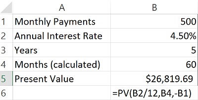
Let's calculate the present value of a 4.5% annuity where regular payments of $500 are made over a period of five years. To determine the present value of that instrument, we use this annuity formula in Excel.
- B1 contains our monthly annuity payment of $500.
- B2 contains the annual interest rate of 4.5%.
- B3 contains the five years we would receive that.
- B4 converts the number of years to months to match the monthly payments.
- =PV(B2/12,B4,-B1) or $26,819.69
- If you buy the annuity for $26,819.69, you receive $30,000 in payments.
PMT - Payment: PMT(rate,nper,pv)
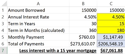
The payment function can be used to calculate the monthly payment on a mortgage or a loan. All you need is the amount borrowed, the annual interest rate and the term of the loan.
In our example:
- B1 contains the amount borrowed $150,000.
- B2 contains the annual interest rate of 4.5%.
- B3 contains the 30 years over which we'd repay the mortgage.
- B4 converts the number of years to months to match the monthly payments.
- =PMT(B2/12,B4,-B1) or a monthly payment of $760.03
The present value (pv) argument is expressed as a negative here because we are, basically, in debt $150,000. Put in your own numbers in the yellow cells and see what you get! Here we entered the same information except the term is 15 instead of 30 years. See the difference in the total interest paid?
NPER - Number of Periods: NPER(rate,pmt,pv)
Each of the functions above has used the NPER argument for number of periods. In this case, it is a function used to determine, for example, how long it would take to pay off a loan, given a known interest rate, monthly payment and loan balance.
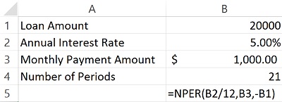
In our example:
- B1 contains the remaining loan amount $20,000.
- B2 contains the annual interest rate of 5%.
- B3 contains the monthly amount we can pay.
- =NPER(B2/12,B3,-B1) or 21 months
Want to see how long it will take you to pay off a debt? Try out your own numbers in the NPER worksheet! You can also upskill further with our Microsoft Excel Training.
Common PMT Errors and How to Fix Them
Even experienced spreadsheet users run into trouble with the PMT function. Here are the three most common errors and how to resolve them:
- PMT returns a negative number. Excel treats payments as cash outflows, so the result is negative by default. To get a positive monthly payment, place a minus sign before the present value argument (e.g., =PMT(B2/12,B4,-B1)) or wrap the entire formula in a negative sign: =-PMT(B2/12,B4,B1).
- Forgetting to divide the annual rate by 12. If your payments are monthly but you enter the full annual interest rate, the result will be dramatically too high. Always divide the rate by 12 for monthly periods, by four for quarterly periods or leave it as-is for annual periods.
- Mismatching period units. The rate and nper arguments must use the same time unit. A common mistake is entering the rate as a monthly figure while leaving nper in years (or vice versa). If your rate is annual and your term is 30 years of monthly payments, use rate/12 for the rate and 30*12 for nper.
Catching these three issues will resolve the vast majority of unexpected results you encounter with the PMT formula. Practicing with additional Excel formulas will sharpen your instinct for spotting similar mistakes across all financial functions.
When to Use PMT vs. Other Financial Functions
The PMT function is just one member of a larger family of Excel finance formulas. The table below shows when to reach for each function.
| Function | What It Calculates | Example Use Case |
|---|---|---|
| PMT | Fixed periodic payment on a loan or investment | Calculate the monthly mortgage payment on a $250,000 home loan |
| FV | Future value of an investment or savings plan | Find out how much $500/month will grow to over 15 years at 3% |
| PV | Present value of a series of future payments | Determine what an annuity paying $500/month for five years is worth today |
| NPER | Number of periods needed to pay off a balance | See how many months it takes to pay off a $20,000 loan at $1,000/month |
| IPMT | Interest portion of a specific payment | Break out how much of payment #24 goes toward interest |
| PPMT | Principal portion of a specific payment | Break out how much of payment #24 goes toward principal |
| RATE | Interest rate per period given the other variables | Back into the rate when you know the payment, term and loan amount |
If you know three of the four core variables (rate, nper, pmt, pv/fv), Excel can solve for the fourth. Choosing the right function simply depends on which variable is missing—whether you are planning a budget, sizing a loan or valuing an investment.
Explore all of these functions and more with Pryor Learning's Microsoft Excel Training.


