Excel Finance Formulas

Given the number-crunching power of Excel, you might surmise that when it comes to calculating money matters, it really shines. And, so it does. In order to understand how the various financial functions, work, there are a few components to understand. Most of the 55 functions that are classified as financial functions in Excel use one or more of the following in their arguments. Some of these are functions in their own right, but all can be arguments in another.

Follow along and try your own numbers out by downloading: Excel Finance Formulas Sample.xlsx

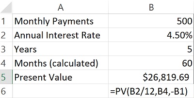
FV – Future Value FV(rate,nper,pmt)

The future value of money is based on an interest rate, regular payments (if any) and a term. For example, if we save $500 per month at 3% annual interest, over a period of 15 years we would have $113,486.34.

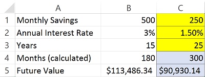
In Excel, we would use the FV function to calculate that, as follows:

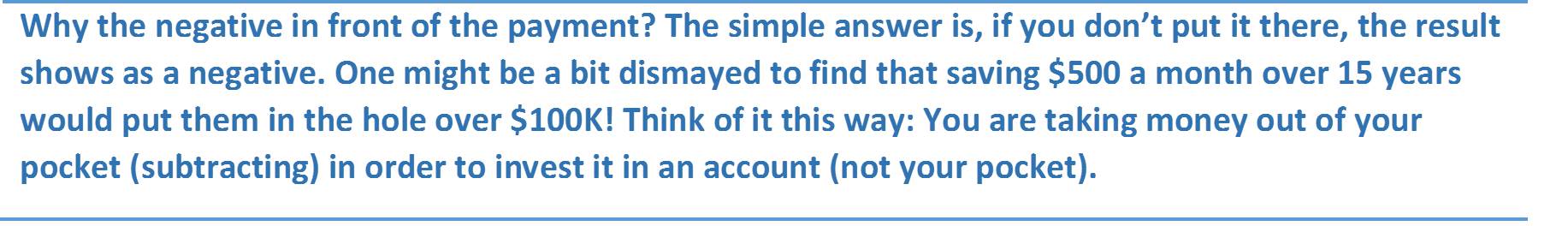
• B1 contains our monthly payment of $500.
• B2 contains the annual interest rate of 3%.
• B3 contains the number of years we would save that.
• B4 converts the number of years to months to match our monthly payments into savings.
• =FV(B2/12,B4,-B1) or $113,486.34
• You invested $90,000 and earned $23,486.34 in interest.

NOTE: Why the “/12?” Well, annual interest rates must be divided by 12 months if the payments will be made monthly. If you have a monthly interest rate, there is no need to do this. However, most interest rates are expressed as annual rates.

In the sample spreadsheet, you’ll find some yellow-shaded cells for you to try out your own calculation! Look for your answers in the blue shaded cells.

PV – Present Value PV(rate,nper,pmt)

Let’s calculate the present value of a 4.5% annuity where regular payments of $500 are made over a period of 5 years. To determine the present value of that instrument, we use this formula.

• B1 contains our monthly annuity payment of $500.
• B2 contains the annual interest rate of 4.5%.
• B3 contains the 5 years we would receive that.
• B4 converts the number of years to months to match the monthly payments.
• =PV(B2/12,B4,-B1) or $26,819.69
• If you bought the annuity for $26,819.69, you would have received $30,000 in payments.

PMT – Payment PMT(rate,nper,pv)

The payment function can be used to calculate the monthly payment on a mortgage or a loan. All you need is the amount borrowed, the annual interest rate and the term of the loan.

In our example:

• B1 contains the amount borrowed $150,000.
• B2 contains the annual interest rate of 4.5%.
• B3 contains the 30 years over which we’d repay the mortgage.
• B4 converts the number of years to months to match the monthly payments.
• =PMT(B2/12,B4,-B1) or a monthly payment of $760.03

The present value (pv) argument is expressed as a negative here because we are, basically, in debt $150,000. Put in your own numbers in the yellow cells and see what you get! Here we entered the same information except the term is 15 instead of 30 years. See the difference in the total interest paid?

NPER – Number of Periods NPER(rate,pmt,pv)

Each of the functions above has used the NPER argument for number of periods. In this case, it is a function used to determine, for example, how long it would take to pay off a loan, given a known interest rate, monthly payment and loan balance.

In our example:

• B1 contains the remaining loan amount $20,000.
• B2 contains the annual interest rate of 5%.
• B3 contains the monthly amount we can pay.
• =NPER(B2/12,B3,-B1) or 21 months

Want to see how long it will take you to pay off a debt? Try out your own numbers in the NPER worksheet!