Conditional Formatting, Excel
Apr 24, 2026
Using Excel Conditional Formatting Based on Another Column or Cell
Key Takeaways
- Excel's built-in conditional formatting presets only format cells based on their own values, but you can use a formula-based rule to format one cell based on another cell's value.
- The key to making conditional formatting based on another column work correctly is using mixed cell references (e.g., $B2) so the formula adjusts row by row but stays locked to the reference column.
- Common use cases include highlighting rows where a status column says "Complete," flagging inventory below a threshold in a separate column or comparing values between two columns.
- Always select your full target range before creating the rule and test with a few rows first to confirm your references are correct.
What Is Conditional Formatting Based on Another Cell?
Standard conditional formatting in Excel evaluates a cell's own value to decide how it should look. For example, you might turn a cell red when its number drops below 20. But what if you want to format one cell (or an entire row) based on the value in a different cell or column? That is conditional formatting based on another cell and it requires a formula-based rule.
Instead of choosing a preset like "Less Than" or "Greater Than," you select "Use a formula to determine which cells to format" in the New Rule dialog and write a formula that points to the reference column. Excel evaluates that formula for each cell in your target range and applies the formatting whenever the formula returns TRUE.
This technique is useful in a wide range of business scenarios:
- Inventory management: Highlight product names or entire rows when a "Units in Stock" column falls below a reorder threshold.
- Task tracking: Format a task description in red when a date column shows the deadline has passed.
- Status-based row highlighting: Shade an entire row green when a "Status" column reads "Complete."
- Data comparison: Flag differences between two columns, such as budget vs. actual spend.
This approach works in Excel 2007 through Microsoft 365 and follows the same general steps in every version. You can find additional techniques and version-specific guidance across our full library of Excel tutorials. If you are new to Excel formulas, Pryor Learning's guide to Excel formula syntax is a helpful starting point.
The Generic Formula for Conditional Formatting Based on Another Cell
Every conditional formatting formula that references another cell follows the same pattern. You select the range you want to format, create a new rule using "Use a formula to determine which cells to format" and enter a formula that points to the reference column.
The generic template looks like this:
=$ReferenceColumn2 = condition
For example, if your data starts in row 2 and you want to format cells in column A whenever column D contains a value greater than 100, your formula would be =$D2>100. The dollar sign before the column letter locks the reference to column D while the row number (2) stays relative so it adjusts for every row in your selected range.
Understanding Mixed Cell References
Getting cell references right is the single most important step when applying conditional formatting based on another column. There are three reference types:
- Relative (B2): Both the column and row shift as the rule moves across cells. This is rarely what you want for cross-column rules.
- Absolute ($B$2): The column and row are both locked. The rule always evaluates the exact same cell no matter where it is applied.
- Mixed ($B2): The column is locked but the row adjusts. This is the reference type you will use most often because it ensures every row checks the correct column while evaluating its own row of data.
When you apply a formula rule across a range, use a mixed cell reference to lock the column reference (e.g., $B2). If you forget the dollar sign before the column letter, Excel will shift the reference sideways as it moves across columns and your rule will evaluate the wrong data.
How to Apply Conditional Formatting in Excel
Steps in this article will apply to Excel 2007-2016. Images were taken using Excel 2016.
Conditional formatting is a useful Excel feature that can help you quickly scan your data without resorting to complicated filtering or building full charts in Excel.
Often, you will use conditional formatting to call attention to cells that represent an outlying condition – such as too many days until delivery or too few items in inventory.
The following example demonstrates Excel's built-in conditional formatting presets, which format a cell based on its own value. If you need to format cells based on a value in a different column, the formula-based approach is covered in the sections that follow.
Here's how to use conditional formatting to show us that an item in our store is getting low on inventory and we will need to re-order soon:
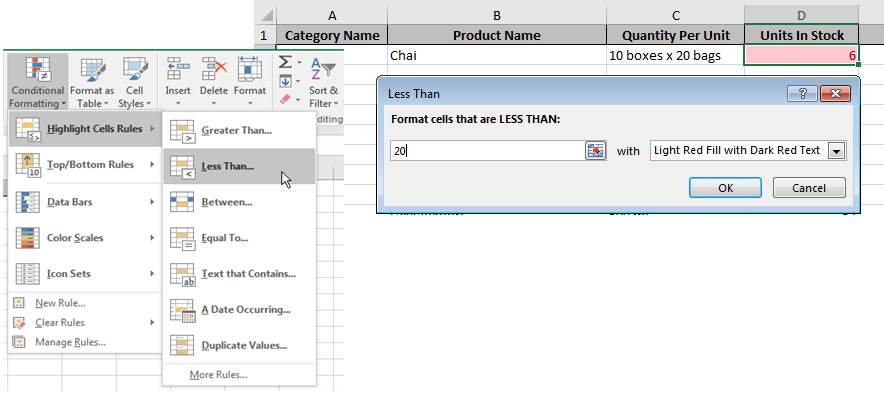
- Highlight the cell in the row that indicates inventory, our "Units in Stock" column.
- Click Conditional Formatting.
- Select Highlight Cells Rules, then choose the rule that applies to your needs. In this example, select Less Than.
- Fill out the Less Than dialog box and choose a formatting style from the dropdown. In our example, we want the cell to change to red background and red text when the cell value is less than 20.
To follow using our example, download 03-Conditional Formatting Across Multiple Cells.xls
I'm sure you have already spotted a problem! There are many rows in our worksheet. Do I have to repeat the above for every cell in the column? Of course, the answer is "no" and Excel gives you a few quick ways to apply conditional formatting to multiple cells.
Select Your Range Before You Begin
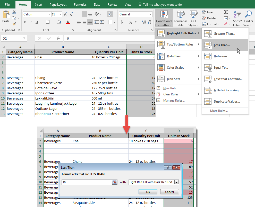
The easiest way to apply conditional formatting to an entire column or row is to select the full target range before you define your rule. To highlight every cell with a value below twenty in our example, your steps would look like this:
- Highlight all of the cells in the sheet to which you'll apply the formatting rules. Do NOT select headings.
- Click Conditional Formatting.
- Select Highlight Cells Rules, then choose the rule that applies to your needs. In this example, select Less Than.
- Fill out the Less Than dialog box and choose a formatting style from the dropdown.
Edit the Rule
If you forget to select your range, or your range changes after you've applied the rule, you can modify it after the rule has been created:
- Place the cursor in any cell to which the conditional formatting rule applies.
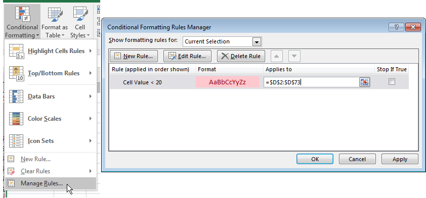
- Click Conditional Formatting, then select Manage Rules.
- Click on the rule you wish to change. (If you don't see your rule, you may not have selected a cell to which the rule applies. Click the Show formatting rules for: dropdown and select This Worksheet to see all rules.)
- Click inside the Applies to field.
- Type the new range of cells, or click the sheet button to click & drag your cursor around the new range of cells. When the Applies to field reflects the correct new range, click OK.
Click and Drag, Copy/Paste
Once a conditional formatting rule has been applied to a cell, the rule will also apply to any cell that is copied from the original. This means you can copy/paste the rule (along with its contents!) and even use the copy handle to drag and copy the rule. Caution! Just like any other formula, you will need to pay attention to your absolute, relative and mixed cell references so that your conditional formatting rules apply correctly. This is especially important when your rule references another column — use a mixed reference like $B2 to lock the column while allowing the row to adjust.
To delete your rule from multiple cells:
- Open the Rules Manager, select the rule and hit Delete Rule
To delete all rules from your sheet:
- Click Conditional Formatting > Clear Rules and select Clear Rules from Entire Sheet
Common Formula Examples for Formatting Based on Another Cell
Now that you understand the mechanics, here are five practical formulas you can use to highlight cells based on another cell value. In each example, assume your data starts in row 2 and you have already selected the target range before creating a new rule with "Use a formula to determine which cells to format."
| Use Case | Formula | What It Does |
|---|---|---|
| Numeric threshold in another column | =$D2<20 | Formats the target cell when column D's value is less than 20 |
| Text match in another column | =$C2="Overdue" | Formats the target cell when column C contains the word "Overdue" |
| Highlight entire row by status | =$F2="Complete" | Applied to a full row range (e.g., $A2:$G100), shades the entire row when column F reads "Complete" |
| Compare two columns | =$A2<>$B2 | Highlights cells where column A and column B do not match |
| Check for blanks in another column | =ISBLANK($E2) | Formats the target cell when column E is empty |
- Numeric threshold in another column — Use =$D2<20 when you want to flag rows where a quantity, score or dollar amount in column D falls below a set number. This is the formula-based version of the inventory example earlier in this article.
- Text match in another column — Use =$C2="Overdue" to change cell color based on another cell value that contains specific text. Swap "Overdue" for any label your data uses.
- Highlight an entire row based on one cell — Apply the rule to a multi-column range like $A2:$G100 and use =$F2="Complete". Because the column is locked with the dollar sign, every cell in the row evaluates the same status column. This is how you achieve conditional formatting for an entire row based on one cell.
- Compare two columns — Use =$A2<>$B2 to spot differences between columns. This is helpful for reconciliation tasks like comparing planned vs. actual values.
- Check for blanks — Use =ISBLANK($E2) to call attention to missing data. This works well for required fields like email addresses or approval dates.
Remember to use mixed cell references in every formula. Lock the column with a dollar sign ($D2) and leave the row relative so the rule evaluates each row independently.
Common Pitfalls and How to Avoid Them
If your conditional formatting based on another cell is not working as expected, check for these common mistakes:
- Using fully relative references instead of mixed references. If you enter =D2<20 instead of =$D2<20, Excel shifts the column reference as the rule moves across cells. The result is that your rule evaluates the wrong column for cells that are not in the first column of your selected range. Always add a dollar sign before the column letter.
- Applying the rule to the wrong range. If you only had one cell selected when you created the rule, the formatting will only appear in that cell. Open the Rules Manager, check the "Applies to" field and expand it to cover your full data range.
- Conflicting rules overriding each other. When multiple rules apply to the same range, Excel processes them in the order listed in the Rules Manager. A rule higher in the list takes priority. If your formatting looks wrong, open the Rules Manager and reorder or delete conflicting rules.
- Extra or missing equals signs in the formula field. The formula field in the New Rule dialog already expects a formula, so you need exactly one equals sign at the start. Entering two (==) or omitting it entirely will cause the rule to fail silently.
Next Steps
Conditional formatting based on another cell is one of the most practical skills you can add to your Excel toolkit. An advanced Excel training program can help you build on this foundation with macros, PivotCharts and other power-user techniques. Download the practice file referenced in this article and try building a few formula-based rules of your own. Once you are comfortable with mixed references, you can move on to advanced techniques like nested formulas, data validation dashboards and dynamic reports.
For more information about how to apply conditional formatting based on formulas and how to highlight entire rows of data, view this article: Get the Most Out of Excel's Conditional Formatting


