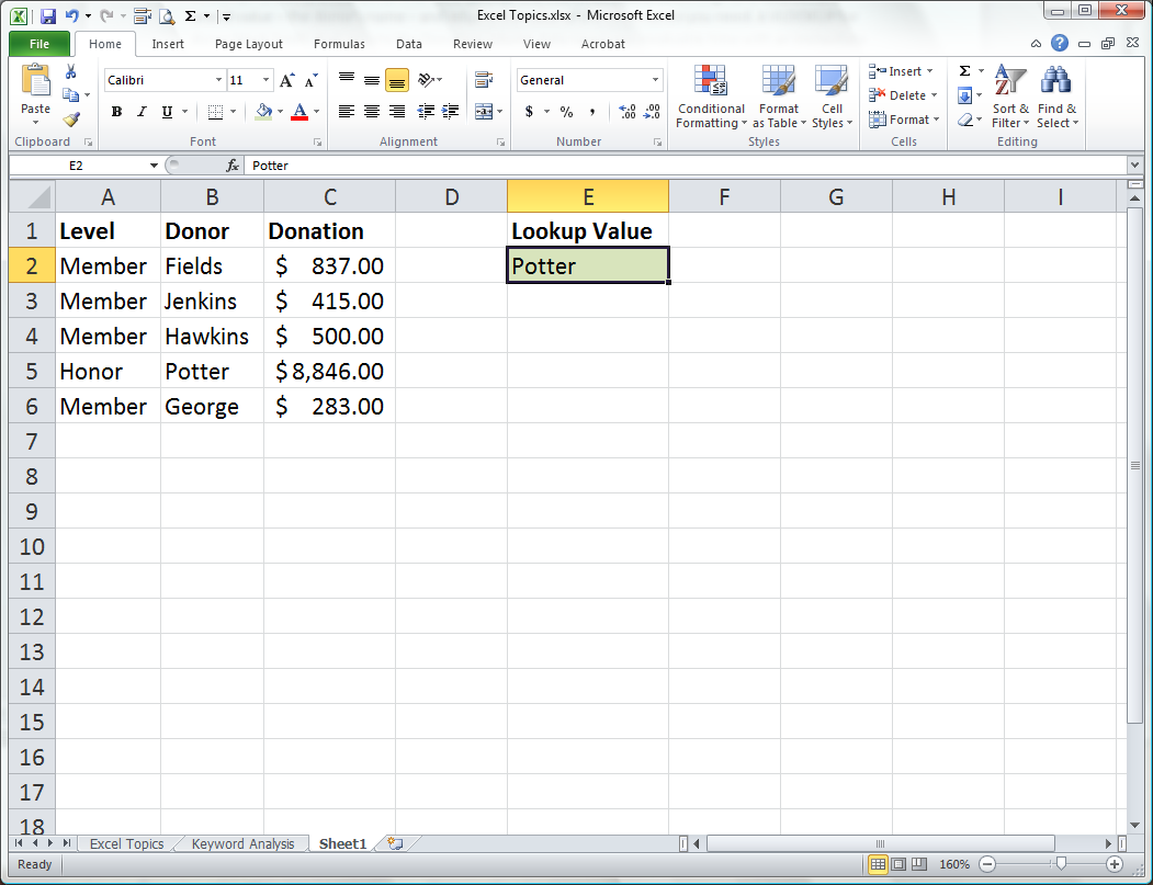
3. Enter a starting value in the field that is referenced by the VLOOKUP function. It should be a value near the top of the data list. In this case, Potter was entered.
4. Select the cell where the VLOOKUP formula will reside. In this example, that is cell F2.
5. In the Formula bar, type =VLOOKUP(
6. Complete the formula as prompted. This helpful tool that shows you the full formula and its variables is called the Formula Autocomplete Tooltip. The components to the VLOOKUP formula and what they represent are detailed below
- The lookup_value is the cell where the searched term is entered. In this example, cell E2 is where the donor’s name is entered.
- The table_array should be the area of data that is searched for the lookup value and the returned value (in this case the donation amount). In this example, that is cells B2 (the top value-containing cell in the Donor column) through C18 (the bottom value-containing cell in the Donation column).
- The col_index_num is the number of the column in the selected array searched for the returned value. Column C is the one searched, and while it is Column 3 in your table (counting from left to right), it is only column 2 of the array you identified for the VLOOKUP. 2 (for Column 2) is entered here.
- The range_lookup value is either TRUE or FALSE. Entering a value of TRUE requires the searched column (the donor column in this example) to be in ascending order, and causes Excel to search for an approximate match. A selection of FALSE eliminates the ascending order requirement but searches only for an exact match. In this example, FALSE is selected.
7. Close the parentheses in the formula.
8. Press the ENTER key on your keyboard.
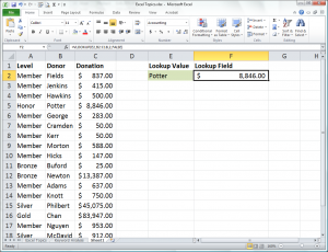
9. Review the result to check your work. =VLOOKUP(E2,B2:C18,2,FALSE)
Practice makes perfect. Try this out on your own and see how quickly you can access the information you need. Just make sure that if you plan to apply your VLOOKUP formula to multiple cells, then your table arguments are absolute references.