Excel
Oct 23, 2023
VLOOKUP vs XLOOKUP, What’s the Difference and When to Use Them
The “new” XLOOKUP function was introduced in Excel 2021 and Office 365, and improves upon the heavily used VLOOKUP function in several ways. Let’s start by reviewing the syntax and an example of each function to understand the differences, starting with VLOOKUP.
VLOOKUP Syntax and Examples
Here is the syntax: VLOOKUP (lookup_value, table_array, col_index_num, [range_lookup])
- lookup_value holds the value or cell reference of the data you know. The value must be located in the first column of the range you specify in the next argument.
- table_array holds the range of cells you want to search. This range must include the lookup value in the first column, and the return value.
- col_index_num holds the column location of the return value. This is specified by column number where 1 is the left-most column of the range entered in the second argument.
- range_lookup is optional and lets you specify whether VLOOKUP should find an approximate or an exact match. Approximate, or TRUE, is the default. FALSE will tell VLOOKUP to return a value only if it finds an exact match in the first column.
We want to use VLOOKUP to find birthday information in an employee database by searching for last names. You might use this to fill out health insurance applications or retirement planning. Here are the important elements of the calculation:
- We will type the name we are looking for in the orange cell, I5 [A]. The VLOOKUP will go in cell J5.
- Our lookup data, Last names, are in Column B, so that will be the leftmost range of our array which also must include the information we want returned [B].
- The information we want is in column D, the 3rd column in our range (not the 3rd in the table)
- We only want to return exact matches.
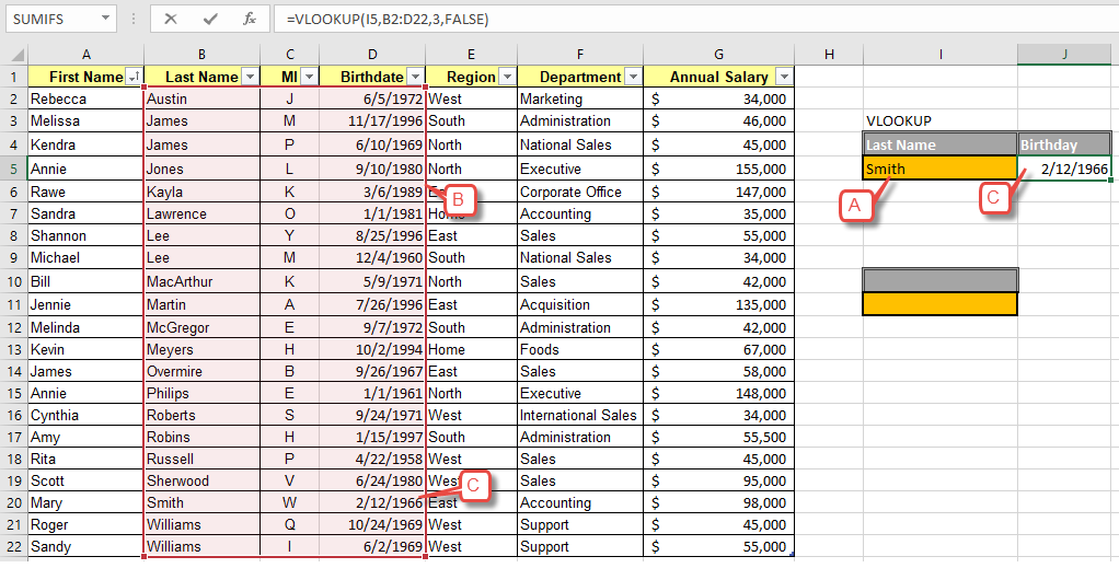 Our function will then be: =VLOOKUP(I5,B2:D22,3,FALSE)When we type the name “Smith” into cell I5, it correctly returns Mary Smith’s birthday [C].
Limitations of VLOOKUP
Here are the limitations of VLOOKUP in this case:
- It assumes that your first array column is sorted. If it is not sorted, you can get wrong results using approximate match.
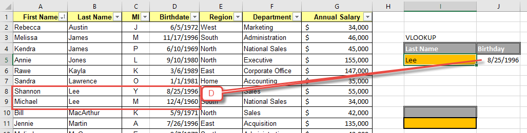
- VLOOKUP can only return the first match it finds. It will not return Michael Lee’s record after returning Shannon Lee [D].
More about VLOOKUP:
- https://www.pryor.com/blog/use-vlookup-to-find-values-from-an-excel-table/
- https://www.pryor.com/blog/using-vlookup-in-an-excel-formula/
XLOOKUP Syntax and Examples
Now let’s look the same example using XLOOKUP. Here is the syntax:
=XLOOKUP(lookup_value, lookup_array, return_array, [if_not_found], [match_mode], [search_mode])
- lookup_value holds the value or cell reference of the data you know.
- lookup_array holds the range of the cells you want XLOOKUP to search.
- return_array holds the range of the location of the return You can specify multiple columns or rows if you wish, but they must be contiguous.
- if_not_found is optional and allows you to specify a custom error message when a search result is not found.
- match_mode is optional allows you to specify how Excel chooses a match. The default is exact match.
- search_mode allows you to specify a search order such as reverse search. The default search starts at the first item.
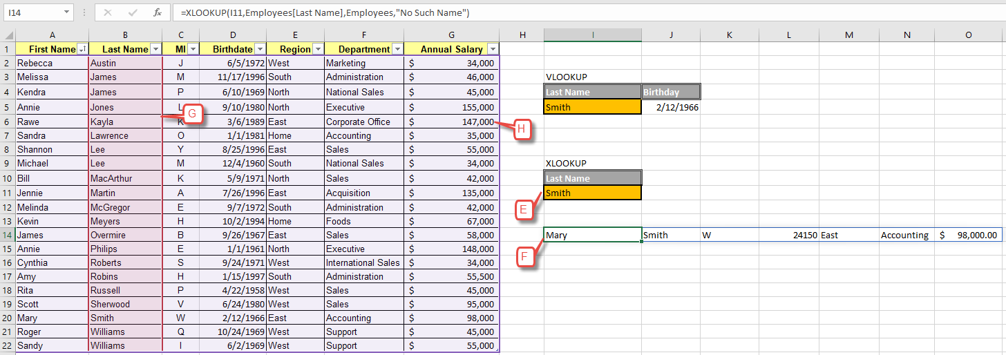
We want to look up complete records for employees by their last name. Here are the important elements of the calculation:
- We will type the name we are looking for in the orange cell, I11 [E]. The XLOOKUP will go in cell I14 [F].
- Our data is in a table named “Employees” and we want to search the Last Name column to find matches.
- We want to return a complete record for each match, so we can specify all columns in the table by using the table’s name: “Employees.” Unlike VLOOKUP, XLOOKUP can return values to the left of the search array.
- We only want exact matches returned.
- We want the text “No Such Name” returned when a match is not found.
- We will leave the match and search mode defaults.
Our function will then be:
=XLOOKUP(I11,Employees[Last Name],Employees,"No Such Name")
Excel helps you view your array arguments by highlighting the lookup_array in red [G], and the return_array in purple [H] when editing your function.
Advantages of XLOOKUP
- XLOOKUP allows you to find matches and return multiple values from the entire record, not just one cell within the record.
- You can also perform both horizonal and vertical lookups whereas before you would have to choose between VLOOKUP (vertical) or HLOOKUP (horizontal).
- XLOOKUP eliminates the dreaded left column lookup limitation of VLOOKUP. This is especially useful when your table changes and the return value is no longer in the same column number.
- XLOOKUP can search in reverse order, bottom to top as well as top to bottom which makes it easier to find the “last” or “first” of items in certain uses.
- Exact match is far more preferred than approximate match. XLOOKUP’s default of exact match is a sigh of relief for many.
- You can customize the error message so that you can tell the difference between a broken function and zero matches.
Disadvantages of XLOOKUP
- Just like VLOOKUP, XLOOKUP can only return the first match it finds. This can cause problems if you have records with the same data in the lookup array.
When to Use VLOOKUP Instead of XLOOKUP?
XLOOKUP is rapidly replacing VLOOKUP and HLOOKUP as a superior option that performs the function of both, better. So, the short answer to this question is don’t. However, the long answer is more nuanced.
XLOOKUP is only available in versions of Excel released after 2021 and is not backward compatible. If you regularly share workbooks with partners who run older software, stick with VLOOKUP so they will be able to use the files.
Similarly, if you are maintaining data that was created pre-2021 using VLOOKUPs, continue to do so. You do not want to introduce mistakes by trying to update working functions when there is no need. If you do decide to reformat an older workbook, make sure you save and archive the original so that you can always return to if your update causes errors.
If you are hesitant to leave your favorite function behind, Pryor Learning has Excel courses available to help you make the leap and stay current with the best that Excel has to offer.


